Financial numeracy and business economics: a free course

A business can grow sales and lose money. A project can show a positive return and still fail to justify its cost. This free course teaches you to identify the units, bases, timing and assumptions behind those conclusions before building a spreadsheet.

Start here: you need basic arithmetic, a calculator and a place to write. No Excel or finance background is required. Work through the nine lessons in order, pause at each check and attempt the final case before opening its solution. The explanations, figures and answer keys are all available on this page.

We use Northstar Bottles, an original fictional business. Unless stated otherwise, figures are USD. Scenario rates and probabilities are teaching assumptions, not current market quotations or forecasts. Each new case states which assumptions apply.

Your outcome: read financial numbers accurately, compare rates, reason about time value, explain unit economics, distinguish relevant costs and support a decision under uncertainty.

1. Read the number before calculating

Northstar Bottles reports revenue of 120 and cash of 35. Is the business large? Can it pay a bill of 20? You cannot tell yet. The numbers need labels. Revenue might be $120,000 for a month, while cash might be $35 million at a year-end. A correct calculation with mismatched labels still answers the wrong question.

By the end of this lesson: you can read a financial number as an amount with a unit, scale, time basis, sign and definition. You do not need a spreadsheet. A pencil and calculator are enough.

Give every number an address

Use six questions before doing arithmetic: What does it measure? In what unit? At what scale? For which date or period? Under what sign convention? Is it an observed amount or an assumption?

Item	Properly labeled value	What it means
Revenue	$120,000 for January	Sales recognized during a month
Cash	$35,000 at January 31	Cash held at one moment
Bottles sold	4,000 in January	A count during a period
Selling price	$30 per bottle	Dollars for each unit
Forecast sales	4,400 bottles for February	An assumption about a future period

Revenue is the amount earned from sales before subtracting expenses. An expense is a cost recognized in measuring profit. Profit is revenue minus the relevant expenses. Cash is money available; cash flow describes receipts and payments over a period. These are related concepts, but their timing can differ.

Northstar can deliver bottles worth $3,000 to a customer in January and receive payment in February. That sale can create January revenue without a January cash receipt. Conversely, collecting an old invoice creates cash without creating a new sale. Later accounting lessons explain recognition rules in more detail; here, the crucial habit is to avoid using “revenue,” “profit” and “cash” interchangeably.

Stocks are snapshots; flows cover intervals

Imagine a water tank. The water inside at noon is a snapshot. Water entering during the next hour is a flow. Opening water plus inflow minus outflow equals closing water. The analogy describes a reconciliation; money has additional accounting categories that water does not.

For cash, the same bridge is:

Closing cash = opening cash + cash received − cash paid.

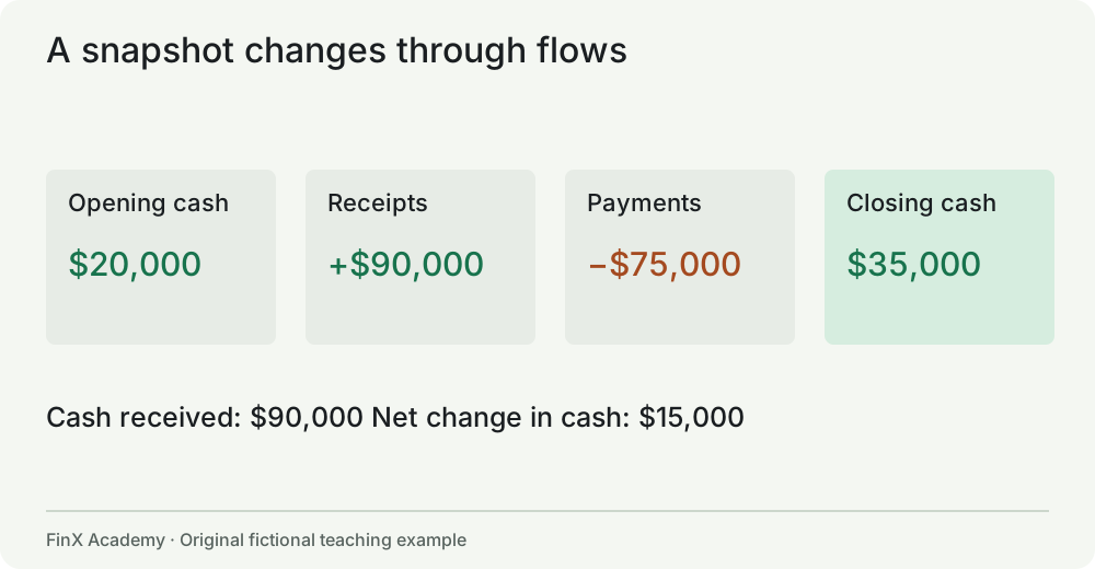
If Northstar starts January with $20,000, receives $90,000 and pays $75,000, it ends with $35,000. Adding the opening and closing balances would not produce “cash generated.” It would add two snapshots. The change in cash is $15,000; receipts are $90,000. Both are useful, but they answer different questions.

Debt, inventory and receivables are also balances measured at dates. Revenue, expenses and cash flow normally cover periods. To compare a balance with a flow, explain the relationship. Inventory divided by annual cost of sales is a fraction of a year, not a profit margin. Multiplying that fraction by days per year converts it into an approximate number of days of inventory.

Scale and units should cancel correctly

“$000” means thousands of dollars. A reported 120 in a $000 table means $120,000. To express it in $millions, divide 120 by 1,000: $0.12 million. Multiplying by 1,000 again would be a million-fold error relative to the correctly converted million-unit figure.

Check an equation through its units: 4,000 bottles × $30/bottle = $120,000. Bottles cancel. By contrast, multiplying a price by revenue creates dollars squared per bottle, which is not revenue. Unit checks often reveal a mistake before a detailed calculation does.

A currency is part of a unit. You cannot add dollars and euros without an exchange-rate convention. At an illustrative rate of $1.10 per euro, €10,000 equals $11,000: euros cancel when multiplied by dollars per euro. The inverse quotation is about €0.9091 per dollar. The two quotations describe the same conversion; multiplying by the wrong one reverses it. The rate here is a fictional teaching input, not a current exchange-rate quote.

Time, signs and precision

Compare January with January, or a complete year with a complete year. A company’s fiscal year need not end in December. Annualizing a quarter by multiplying by four is an assumption about the remaining quarters, not a fact. It can be misleading for a seasonal business.

State whether payments are positive amounts that you subtract or negative cash flows that you add. Both conventions work. Mixing them subtracts an outflow twice. Parentheses such as (75) often denote a negative amount, but read the table’s convention. A dash can mean zero, unavailable or not applicable; a blank is not automatically zero.

Keep sufficient precision during calculations and round the final display. Reporting a forecast to the nearest cent does not make its assumptions accurate. A sensible answer combines reproducible arithmetic with an honest level of precision.

Check yourself

1. A table in $000 shows cash of 275. What is that amount in dollars and in $millions?
2. Opening cash is 35,000. Receipts are 110,000 and payments are 98,000. What is closing cash?
3. A January sales figure is compared with cash at January 31. Why is subtracting one from the other not a measure of profit?

Answers and reasoning

1. $275,000; $0.275 million. Identify the starting scale before converting.
2. $47,000 = $35,000 + $110,000 − $98,000. The $12,000 change is not the same as receipts.
3. Sales is a flow and closing cash is a stock. Profit requires the expenses associated with the period; cash also reflects collection/payment timing and financing or investing flows.

Transfer task: find a financial table and annotate one number with its unit, scale, date or period, definition and sign. If a label is missing, state the question you would ask instead of guessing.

2. Percentages, ratios and weighted averages

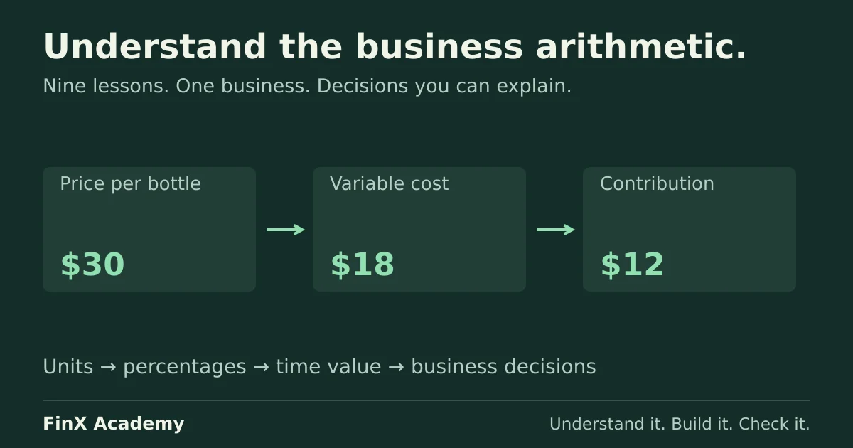
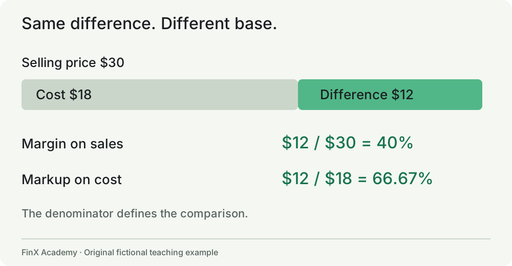
Northstar buys a bottle for $18 and sells it for $30. The difference is $12. One colleague calls that a 40% margin; another calls it a 66.7% markup. Both can be right. They are dividing by different amounts.

By the end of this lesson: you can identify the base of a percentage, explain percentage-point changes, convert between margin and markup, and aggregate ratios with suitable weights.

A percentage is a ratio with a named base

Percent means “per hundred.” The decimal 0.08, fraction 8/100 and percentage 8% represent the same proportion. Eight percent of $250 is 0.08 × $250 = $20. To find the percentage represented by $20 out of $250, divide: 20/250 = 0.08 = 8%.

The denominator is the base. Label it before calculating. “Costs are 60%” is incomplete. Sixty percent of revenue? Of last year’s costs? Of the budget? Percentages become meaningful only after the comparison is specified.

For a change between two positive amounts:

Percentage change = (new amount − old amount) / old amount.

Sales rising from $100,000 to $120,000 increase by $20,000, or 20% of the original $100,000. Reversing that move is a decline of 20,000/120,000 = 16.67%, because the starting base has changed. A 20% rise followed by a 20% fall takes 100 to 120 to 96. It does not return to 100.

If the old value is zero, the standard percentage-change calculation is undefined. Report the absolute change and the starting point. If profit moves from a loss of $10,000 to a profit of $5,000, division by the negative base gives −150%, which is easily misread. Say “a $15,000 improvement, from a loss to a profit” and explain the crossing of zero. Do not hide these cases behind a convenient zero result.

Percentage points and basis points

A margin increases from 20% to 25%. Its change is 5 percentage points, or 500 basis points. One basis point is one hundredth of a percentage point: 0.01 percentage point, or 0.0001 as a decimal.

The relative increase in the margin is 5/20 = 25%. These statements answer different questions. “Margin increased five percent” is ambiguous: it could mean 20% became 21%, or someone might incorrectly intend 25%. Write “five percentage points” when subtracting two percentage levels.

Margin and markup: same dollars, different denominator

Calculation	Formula	Northstar example
Difference per bottle	Price − relevant cost	$30 − $18 = $12
Margin on sales	Difference / selling price	$12 / $30 = 40%
Markup on cost	Difference / cost	$12 / $18 = 66.67%

The word “margin” also needs a definition. Gross margin normally uses revenue minus cost of goods sold. Operating margin includes operating expenses. Contribution margin subtracts costs that vary with activity. Our $18 is the variable cost in this teaching case; its contribution margin is 40%. Do not call it gross margin in a real business without checking which costs are included.

If a product costs $80 and needs a 20% margin on sales, the price is 80/(1 − 0.20) = $100. Multiplying cost by 1.20 gives $96, a 20% markup and a margin of 16/96 = 16.67%. The mistaken price looks plausible because the arithmetic is correct; the denominator answers the wrong question.

For positive prices and costs, margin = markup/(1 + markup), and markup = margin/(1 − margin). These conversion formulas follow from price = cost + difference. They do not remove the need to define which costs you mean.

Why averaging percentages often fails

Northstar has two channels:

Channel	Revenue	Contribution	Contribution margin
Direct	$90,000	$36,000	40%
Wholesale	$10,000	$2,000	20%
Total	$100,000	$38,000	38%

The simple mean of 40% and 20% is 30%. It gives a small channel the same importance as a large one. The business margin is total contribution divided by total revenue: 38,000/100,000 = 38%.

Equivalently, weight each margin by its share of revenue: 40% × 90% + 20% × 10% = 38%. The denominator tells you the weight. Revenue weights aggregate margins; units sold weight average selling prices. If one channel sells 100 bottles for $30 and another sells 300 for $20, the average selling price is (100 × 30 + 300 × 20)/400 = $22.50, not $25.

A mix shift can change the total margin even when neither channel changes its own margin. If the two channels each provide $50,000 of revenue, the overall margin becomes 30%. That decline is a composition effect, not proof that unit economics worsened within each channel.

Check yourself

1. A rate rises from 4.25% to 4.75%. State the percentage-point and basis-point changes.
2. A product costs $60 and needs a 25% margin on sales. What price achieves it?
3. Segment A has $200 of revenue and a 10% margin; B has $800 and a 30% margin. What is the combined margin?

Answers and reasoning

1. 0.50 percentage point, or 50 basis points. The relative rise is about 11.76%, a different measure.
2. $80 = 60/0.75. The $20 difference is 25% of the $80 selling price.
3. 26%. Contribution is 20 + 240 = 260; divide by total revenue of 1,000. A simple 20% average gives equal weight to unequal denominators.

Transfer task: rewrite “profitability improved by 10%” as two precise possible statements, then name the additional information needed to know which was intended. For formula-specific practice later, use the percentage-change guide.

3. Growth and compounding

Revenue rises 50% in one year and falls 50% the next. The average of the two rates is zero. Yet $100 becomes $150 and then $75. The business ends smaller. Averages and compounded outcomes are measuring different things.

By the end of this lesson: you can chain growth rates, calculate a compound annual growth rate, distinguish that rate from an arithmetic mean, and identify when annualization is unjustified.

Growth works through multipliers

An increase of 10% multiplies a value by 1.10. A decline of 10% multiplies it by 0.90. For successive periods, multiply the factors:

Ending value = starting value × (1 + g₁) × (1 + g₂) × …

Northstar’s annual revenue of $120,000 grows 10% and then 20%. It becomes $132,000, then $158,400. The total growth is 1.10 × 1.20 − 1 = 32%, not 30%. The second year’s increase applies to the already enlarged base.

Imagine stacking blocks, with each new layer sized as a proportion of the whole stack already present. The base for the next layer grows. This is compounding. The analogy does not imply that businesses must grow: negative rates shrink the stack, and real business drivers can change.

Simple growth versus compound growth

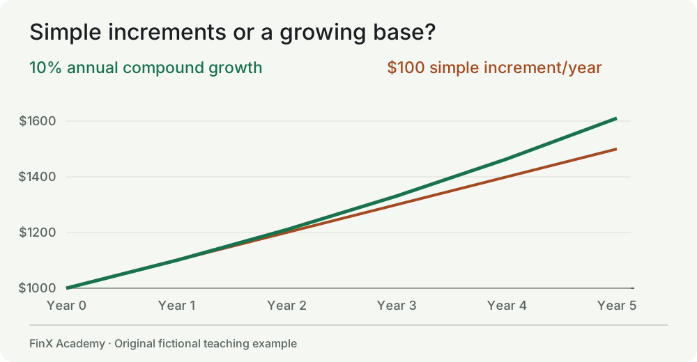
With simple growth, the increment is calculated on the original amount each time. At 10% on an original $1,000, three annual increments of $100 produce $1,300. With annual compounding, the path is $1,000 → $1,100 → $1,210 → $1,331.

The compound formula for a constant rate is ending value = beginning value × (1 + g)ⁿ, where n is the number of periods. A monthly rate needs a count of months. An annual rate needs a count of years or an explicitly defined fractional-year convention.

CAGR is the smooth rate connecting two endpoints

Suppose revenue grows from $100,000 at the end of Year 0 to $133,100 at the end of Year 3. The constant annual rate that links them is:

CAGR = (ending value / beginning value)^(1 / number of years) − 1.

Here, (133,100/100,000)^(1/3) − 1 = 10%. There are three intervals between four year-end observations. Counting observations rather than intervals would understate the rate.

CAGR summarizes endpoints; it does not describe every year’s experience. Both 100 → 110 → 121 → 133.1 and 100 → 150 → 90 → 133.1 have a 10% three-year CAGR. Their volatility, financing needs and operating problems are different. Always inspect the path as well as the endpoint.

For positive values, the compound average is the geometric mean of the growth factors minus one. In the +50%, −50% example, √(1.50 × 0.50) − 1 is about −13.40% a year. Applying that rate twice produces the same $75 endpoint. The zero arithmetic mean describes the average of the two observed rates, not the realized compounded result.

Recovery takes a different percentage

After a 25% decline, 100 becomes 75. Returning to 100 requires 25/75 = 33.33% growth. After a 50% decline, the required recovery is 100%. For a decline d between zero and one, the recovery rate is d/(1 − d). At a complete loss, no finite percentage increase on zero restores the original amount.

This is another denominator problem. It does not mean gains and losses are treated unfairly; the base has changed. The calculation matters whenever a performance chart or a growth narrative combines positive and negative periods.

Annualization is a model assumption

A 2% monthly rate repeated for twelve months produces (1.02)¹² − 1 = 26.82%, not 24%. Multiplying by twelve is a simple annualization; compounding assumes each month’s percentage applies to the updated base.

But a single month of 2% sales growth does not establish that the same rate will repeat. Seasonality, capacity, customer churn and unusual orders can make the extrapolation unrealistic. Similarly, annualizing a strong fourth quarter can overstate a seasonal business’s annual revenue.

Standard CAGR is usually inappropriate when the beginning value is zero or the series crosses zero. A loss becoming a profit is not well explained by taking a fractional power of a negative ratio. Report absolute changes, the crossing of zero and the operating explanation. For an investment with contributions or withdrawals, account-value CAGR also mixes external cash flows with performance; a later returns lesson treats that separately.

Check yourself

1. Revenue rises 20% and then falls 10%. What happens to an initial $200?
2. A metric rises from 80 to 125 over two years. What is its CAGR?
3. Sales were 100, 200 and 121 at three successive year-ends. Why is “10% annual growth” incomplete?

Answers and reasoning

1. $216, from 200 × 1.20 × 0.90. Total growth is 8%.
2. 25%, because √(125/80) − 1 = 0.25. Check by multiplying 80 by 1.25 twice.
3. The two-year CAGR is 10%, but the path includes a 100% rise followed by a 39.5% decline. The smooth rate hides the intermediate volatility.

Transfer task: sketch two different three-year paths with the same starting and ending values. Explain which could place greater pressure on cash, and why endpoint growth alone cannot answer that question. The CAGR guide adds spreadsheet implementation after the idea is clear.

4. Money through time

Would you rather receive $1,000 today or $1,100 in a year? The larger number is not enough to decide. You need to compare both amounts at the same date, using a suitable rate and consistent assumptions about risk and purchasing power.

By the end of this lesson: you can calculate future and present value, match rates to periods, distinguish a quoted nominal rate from an effective rate, and avoid mixing nominal and real cash flows.

Draw the timeline first

Label today as time zero. Put the future payment at the end of Year 1. Assume, for this example, that an appropriate annual rate for these comparable cash flows is 8%. This is a teaching assumption, not a recommended investment return or a current market rate.

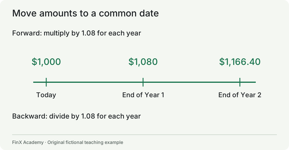
At 8%, $1,000 today is equivalent to $1,080 in one year. The offered $1,100 is $20 larger at that future date. Alternatively, bring the offer back to today: $1,100/1.08 = $1,018.52. Under the stated assumptions it is worth $18.52 more today than $1,000.

Think of the timeline as a ruler. You cannot compare lengths measured from different starting points without aligning them. Discounting aligns financial amounts to a common date. The analogy is limited: the appropriate discount rate is an economic assumption, not a physical constant.

Future value = present value × (1 + r)ⁿ.

Present value = future value / (1 + r)ⁿ.

The rate r and number of periods n must refer to the same interval. Discounting is the reverse of compounding. If you discount $1,166.40 received in two years at 8%, you get $1,000; compounding that $1,000 at 8% for two years gets you back to $1,166.40.

With positive discount rates, a later payment has a smaller present value. At a zero rate, timing does not change the arithmetic value. Negative rates reverse that particular relationship. Different risks, currencies or restrictions can require different assumptions; comparing face amounts alone is insufficient.

Multiple payments need multiple time labels

Suppose Northstar expects $500 at each of the next two year-ends. At 8%, their combined present value is 500/1.08 + 500/1.08² = $891.63. Dividing the $1,000 total by 1.08² incorrectly treats both payments as arriving at the end of Year 2.

For a constant payment C at the end of each period for n periods, the annuity shortcut is PV = C × [1 − (1 + r)⁻ⁿ]/r when r is nonzero. An annuity is simply a regularly spaced stream of equal payments. At a zero rate, use C × n. Payments made at the beginning of periods occur one interval earlier and have a different present value. For irregular dates, use explicit dates and a stated convention rather than pretending every gap is a year.

A perpetuity is the idealized limiting case of equal payments continuing indefinitely. If the first payment arrives one period from now and the constant discount rate is positive, PV = C/r. The shortcut relies on those assumptions; it is not a claim that an actual business payment is guaranteed forever.

Quoted rates and effective rates

An annual nominal rate of 12% compounded monthly specifies a monthly rate of 12%/12 = 1%. The effective annual rate is (1.01)¹² − 1 = 12.68%. It includes the effect of monthly compounding.

If 12% is already an effective annual rate, dividing it by twelve does not produce the equivalent compound monthly rate. That rate is (1.12)^(1/12) − 1 ≈ 0.9489%. Read the quotation before converting. Fees and legal lending disclosures add further considerations outside this introductory example.

“Nominal” has another use: amounts measured in money of the relevant future date, including inflation. Do not confuse that meaning with a nominal quoted interest rate. Always state which meaning applies.

Nominal money and real purchasing power

If your money grows 8% while prices rise 3%, your purchasing-power growth is 1.08/1.03 − 1 = 4.85%, not exactly 5%. Subtraction is an approximation. The exact relationship is 1 + nominal return = (1 + real return) × (1 + inflation).

Use nominal cash flows with a nominal discount rate and real cash flows with a real rate. If a $1,000 amount in today’s purchasing power becomes $1,030 nominal cash in a year, discounting $1,030 at 8% gives $953.70. Discounting the real $1,000 at 4.8544% gives the same result. Mixing the real cash with the nominal rate understates this value.

Check yourself

1. What is the present value of $1,210 received in two years at 10% annually?
2. What is the effective annual rate for 6% nominal annual interest compounded monthly?
3. Why is $100 today plus $100 in a year not the same as $200 today at a positive discount rate?

Answers and reasoning

1. $1,000 = 1,210/1.10². Check by compounding forward.
2. About 6.17% = (1 + 0.06/12)¹² − 1. Each month earns interest on the updated balance.
3. The second $100 is received later and must be discounted to compare at today’s date. At 10%, the combined present value is $190.91.

Transfer task: draw the payment dates before touching the calculator. Write the rate convention beneath the timeline. This single habit prevents many timing errors in a later model.

5. NPV, IRR and investment decisions

Northstar can buy a machine for $60,000 today. The teaching forecast says it will generate $36,000 of incremental net cash at each of the next two year-ends, with no remaining value. Total future cash is $72,000. Is the $12,000 undiscounted surplus enough to justify the machine?

By the end of this lesson: you can calculate net present value, interpret an internal rate of return, and explain why timing, scale and incremental cash flows matter. You are learning a decision method, not receiving an investment recommendation.

NPV puts every cash flow at one date

At an assumed 8% annual required return:

Time	Incremental cash flow	Discount factor	Present value
Today, t = 0	−$60,000	1.000000	−$60,000.00
End of Year 1	$36,000	1/1.08	$33,333.33
End of Year 2	$36,000	1/1.08²	$30,864.20
Total	$12,000 undiscounted		$4,197.53 NPV

Net present value (NPV) = the sum of all cash flows discounted to time zero, including the initial outflow.

The positive $4,197.53 is the forecast value above the 8% required return, expressed in today’s dollars. It is not an extra cash payment, an accounting profit or a guaranteed gain. A zero NPV means the projected cash flows exactly compensate for the assumed required return. A negative NPV means they fall short under those assumptions.

Do not discount the initial outflow for an extra year. It occurs today. Likewise, do not omit it simply because the future inflows look attractive. For spreadsheet implementation later, note that some functions discount their first listed amount by one period; the economic timeline remains the authority.

“Incremental” means caused by the decision

Compare the business with the machine against the business without it. Include the purchase, changes in cash operating costs, taxes when relevant, extra inventory or receivables, and eventual proceeds or cleanup costs. Depreciation is not itself a cash payment, though it can affect taxes. Do not confuse accounting earnings with project cash flow.

The simple $36,000 example already represents net incremental cash. Adding savings again would count the same benefit twice. If the project delays collections, profitable sales can also require cash tied up in receivables. If cash is recovered at the end, place that release on the timeline explicitly.

A project discounted using a rate that already reflects financing should not also subtract the same financing cost indiscriminately from the cash flow. Detailed financing and tax conventions belong in corporate finance; for this lesson, use the stated unlevered project cash flows and rate consistently.

IRR is the rate that makes NPV zero

The internal rate of return is a rate inferred from the project’s cash flows. For this machine it is approximately 13.07%. At that rate, the present value of the two $36,000 receipts equals $60,000.

For a conventional project with one initial outflow followed by inflows, an IRR above the appropriate required return agrees with positive NPV. The rate is a summary, not a promise. It also does not tell you how many dollars of value the project creates.

Consider two mutually exclusive one-year projects at an 8% required return:

Project	Cost today	Cash in one year	IRR	NPV
Small	$100	$120	20%	$11.11
Large	$1,000	$1,150	15%	$64.81

Small has the higher percentage return. Large creates more projected dollar value. If both are feasible alternatives with the stated comparable risks and no other constraints, NPV favors Large. If capital is constrained, you must evaluate the feasible combination of projects; neither “highest IRR” nor “largest individual NPV” mechanically solves every allocation problem.

Some cash-flow patterns have more than one IRR. The sequence −100, +230, −132 has NPVs of zero at both 10% and 20%. Others have no useful IRR. Multiple sign changes are a warning to inspect the NPV profile and the economics, not a reason to trust whichever root a calculator returns.

Payback answers a narrower question

Simple payback asks how long cumulative undiscounted receipts take to cover the initial cost. For the machine, $36,000 has been recovered after Year 1. If Year 2’s cash arrives evenly, the remaining $24,000 takes 24,000/36,000 = two thirds of that year: about 1.67 years. Under the original assumption that cash arrives only at year-end, recovery occurs at the end of Year 2. The timing convention changes the answer.

Payback can describe liquidity exposure, but it ignores the required return and cash flows after the cutoff. Discounted payback fixes the first weakness, not the second. A project that repays quickly can still destroy value if later costs are large.

Check yourself

1. Pay $1,000 today and receive $1,100 in one year. At an 8% required return, what are NPV and IRR?
2. Why does increasing the required return reduce NPV for a conventional outflow-then-inflows project?
3. A $5,000 research bill was paid last month and is nonrefundable. Should it be subtracted again when deciding whether to buy the machine now?

Answers and reasoning

1. NPV $18.52; IRR 10%. NPV uses the specified 8% rate; IRR solves for the rate that produces zero NPV.
2. Future positive cash flows receive smaller present-value weights while the time-zero outflow remains unchanged.
3. No: it is a sunk cost that does not change between the alternatives now. Include any additional research spending that the decision would cause. Lesson 7 develops that distinction.

Transfer task: explain a positive NPV to a manager without using the phrase “total profit.” Identify the one assumption you would investigate first. The NPV guide provides a later spreadsheet treatment.

6. Revenue, costs and break-even

Northstar sells 4,000 bottles a month for $30 each. Variable cost is $18 per bottle. Fixed operating costs are $36,000 a month within the current operating range. The business earns $12,000 of monthly operating profit in this simplified model, before interest and tax.

By the end of this lesson: you can build this economic relationship without a spreadsheet, calculate break-even and target profit, and explain operating leverage and capacity limits.

Build the business from its drivers

Line	Relationship	Base month
Revenue	Price × units sold	$30 × 4,000 = $120,000
Variable costs	Variable cost per unit × units sold	$18 × 4,000 = $72,000
Contribution	Revenue − variable costs	$48,000
Fixed operating costs	Monthly amount within relevant range	$36,000
Operating profit	Contribution − fixed costs	$12,000

Each bottle contributes $12 toward fixed costs and then profit. Imagine each sale dropping twelve dollars into a jar that must first cover a thirty-six-thousand-dollar bill. Until the bill is covered, contribution reduces the loss. Afterward, additional contribution increases operating profit. The jar is an analogy for the model; real cash can arrive later than the sale.

Contribution margin per unit = price − variable cost per unit. Contribution margin ratio = contribution/revenue. Here, the ratio is 40%. Contribution is not the final profit: rent, salaried staff and other fixed costs still need to be covered.

Fixed and variable are behavior descriptions

A variable cost changes with activity in this model. A fixed cost stays constant within a defined period and relevant range. “Fixed” does not mean permanent. Adding a second shift or facility can raise the fixed-cost base. A mixed cost includes a fixed component and a variable component, such as a service contract plus a charge per order.

The distinction depends on the decision and horizon. Labor can be fixed over a short committed schedule but adjustable over a longer planning period. Shipping may vary per order, not per bottle. Model the actual driver instead of forcing every cost into “per unit sold.”

Production and sales are also different quantities. If Northstar makes 4,500 bottles and sells 4,000, inventory changes. The simple example assumes production equals sales, no inventory complications, unchanged prices and variable unit costs, and sufficient capacity. State those assumptions before using the result.

Break-even and target profit

Set operating profit to zero:

Break-even units = fixed costs / contribution per unit.

Northstar breaks even at 36,000/12 = 3,000 bottles, or $90,000 revenue. The revenue version is fixed costs/contribution margin ratio: 36,000/0.40 = 90,000. Check the answer: 90,000 − 54,000 − 36,000 = zero.

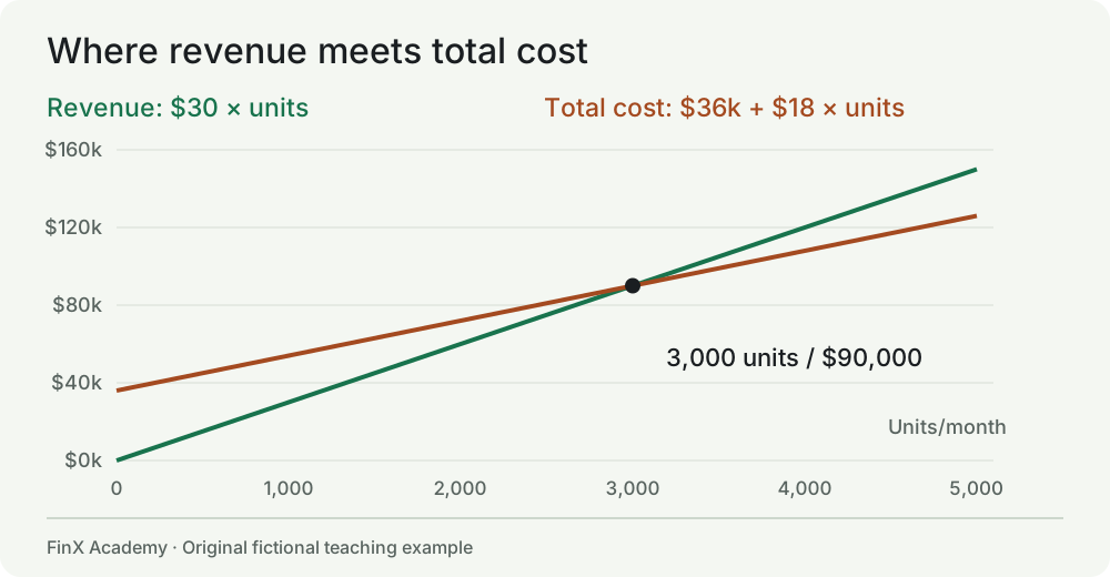
To target $18,000 of operating profit, required units are (36,000 + 18,000)/12 = 4,500. If units cannot be fractional, round the required quantity upward. This model targets pretax operating profit; a target after tax requires a consistent tax treatment.

If contribution per unit is zero or negative while fixed costs are positive, there is no finite positive break-even volume under the unchanged model. More sales do not repair that relationship. Price, variable cost or fixed cost must change.

At 4,000 units, the margin of safety is 1,000 units, or 25% of actual volume: (4,000 − 3,000)/4,000. It describes how far modeled sales could fall before operating profit becomes zero, assuming the other inputs stay constant. It is not a probability of failure.

Why profit changes faster than sales

Increase volume by 10%, from 4,000 to 4,400, holding price and costs constant. Revenue rises from $120,000 to $132,000. Contribution rises from $48,000 to $52,800. Fixed costs stay $36,000, so profit rises from $12,000 to $16,800: a 40% increase.

At the base point, degree of operating leverage = contribution/operating profit = 48,000/12,000 = 4. Under this linear, unchanged-cost structure, a 10% volume-driven sales change creates a 40% profit change from that base. The same mechanism magnifies a fall. Near break-even, the ratio becomes very large; at zero profit it is undefined. Do not apply it mechanically across step-cost changes or price/mix changes.

Capacity and sales mix can change the answer

Suppose current capacity is 4,200 units. A target of 4,500 units is mathematically sufficient but operationally impossible without a change. If expanding capacity adds $6,000 of monthly fixed cost, recalculate using $42,000 of fixed costs. The new target volume for $18,000 profit is 5,000 units. Then check whether the expansion actually provides that capacity.

In a business with multiple products, break-even depends on the sales mix. A weighted contribution assumes a stable mix. If low-contribution sales replace high-contribution sales, the old break-even estimate becomes unreliable. Link quantity, price, mix and capacity explicitly.

Check yourself

1. If variable cost rises to $20 while price stays $30 and fixed costs remain $36,000, what is break-even volume?
2. At those revised costs, what profit does 4,000 units produce?
3. In the original model, can Northstar reach $18,000 profit at a capacity of 4,200 units?

Answers and reasoning

1. 3,600 units, from 36,000/(30 − 20).
2. $4,000, from 4,000 × $10 − $36,000. A $2 unit-cost increase removes $8,000 of profit at that volume.
3. No. It needs 4,500 units with unchanged economics. At 4,200 units it earns $14,400. Any capacity expansion must include its incremental costs.

Transfer task: explain why a 10% increase in price and a 10% increase in volume do not have the same profit effect. Under the original assumptions, the price increase adds $12,000 of profit at 4,000 units; the volume increase adds $4,800. Real price changes may also change demand.

7. Relevant costs and constrained decisions

Northstar receives a special order for 500 bottles at $24 each, below the normal $30 price. Variable production cost is $18 per bottle. Should it reject the order because the price is below its fully allocated cost? Or accept because every bottle contributes $6? Both shortcuts can fail.

By the end of this lesson: you can identify costs and benefits that change between alternatives, recognize opportunity cost, and evaluate a decision with a scarce resource.

Compare two futures from today

A relevant amount changes because of the decision. A sunk cost has already been incurred and cannot be changed by the current choice. An opportunity cost is the value of the best feasible alternative you give up.

Northstar paid a nonrefundable $2,000 design fee last month. Accepting or rejecting the order today does not recover that payment. It is sunk. However, a new $1,000 setup charge incurred only if the order is accepted is relevant. A common expense allocated to the order is not automatically avoidable; ask whether total cash outflow changes if the order is rejected.

Imagine choosing which customer gets the last available seat on a bus. An empty seat can be filled without displacing anybody. A full bus forces you to give up another passenger’s fare. Capacity changes the decision. A production line is more complicated than a bus, but the same opportunity-cost principle applies.

Case A: genuinely spare capacity

Assume Northstar has spare capacity for all 500 bottles, the sale does not affect regular customers or future pricing, and there are no extra costs beyond the $18 variable cost and $1,000 setup fee.

Incremental item	Calculation	Amount
Order revenue	500 × $24	$12,000
Variable cost	500 × $18	−$9,000
Setup cost	Incurred only if accepted	−$1,000
Incremental operating benefit	Total	$2,000

Under those assumptions, the order improves operating profit by $2,000. The earlier design fee does not change the accept/reject comparison. Existing fixed costs that continue either way do not become avoidable merely because an allocation spreadsheet assigns some of them to this order.

The relevant minimum price is $18 + $1,000/500 = $20 per bottle for this particular short-run order. That is not a sustainable general pricing strategy. A business must cover its long-run capacity and other costs across its activities. A short-run incremental decision and a long-run price policy are different questions.

Case B: the order displaces regular sales

Now assume there is no spare capacity. Each special-order bottle displaces a regular bottle that would have contributed $30 − $18 = $12. The opportunity cost is 500 × $12 = $6,000.

The order’s $2,000 direct benefit minus the $6,000 contribution forgone equals −$4,000. The exact same price and variable cost now imply a worse choice. Relevant minimum price becomes $18 + $2 setup cost per bottle + $12 contribution forgone = $32. That threshold depends on the stated one-for-one displacement and cost assumptions.

Do not subtract both the displaced sale’s full revenue and its contribution. Using contribution already accounts for the variable costs saved when those regular units are not produced. Double-counting opportunity cost can be as misleading as ignoring it.

A bottleneck changes what to maximize

Suppose product A contributes $12 per unit and uses two machine minutes. Product B contributes $9 and uses one minute. With machine time as the only bottleneck, A earns $6 per minute, while B earns $9 per minute.

Product	Contribution/unit	Minutes/unit	Contribution/minute
A	$12	2	$6
B	$9	1	$9

With 100 available minutes and enough demand for either product, producing only A gives 50 units and $600 contribution. Producing only B gives 100 units and $900. Ranking by contribution per unit would choose incorrectly. Rank by contribution per unit of the scarce resource, then respect demand limits and any other constraints. Multiple bottlenecks, minimum orders and setup costs can require a more complete optimization model.

Incremental, average and marginal are different

Average cost divides total cost by units. Incremental cost measures the total cost change caused by a choice. Marginal cost concerns one additional unit at the current operating point. A step cost makes “one more” potentially expensive: the first unit beyond current capacity may require another shift.

Before deciding, ask whether the proposed action changes customer behavior, quality, delivery reliability, credit risk or future prices. These effects may matter even when the simple model does not quantify them. Record unresolved assumptions rather than assigning invented precise values.

Make or buy: reconcile the whole business

An outsourcing quote should be compared with the manufacturing costs actually avoided, any new delivery, inspection and transition costs, and the value of released capacity. An allocated head-office charge is not a saving if the bill continues after outsourcing. Conversely, a fixed lease can be relevant if it can be cancelled or sublet. State the time horizon: a cost that cannot change this month might be avoidable next year.

Closing a department presents the same issue. Remove its lost revenue and the costs that genuinely disappear, then account for the alternative use of people, space and equipment. Reconcile the change in the whole business. The department’s reported loss after common-cost allocations is not enough to establish the effect of closing it.

Demand and pricing belong in the model

Higher price increases contribution per unit if variable cost is unchanged, but customers may buy fewer units. Price elasticity of demand describes the proportional quantity response to a proportional price change. The denominator convention matters; the midpoint method uses the average of the two prices and the average of the two quantities.

For example, price rises from $30 to $33 while observed quantity falls from 4,000 to 3,600. Under the midpoint method, quantity changes by −400/3,800 = −10.53%, and price changes by 3/31.5 = 9.52%. Their ratio is about −1.11. Revenue falls from $120,000 to $118,800, yet contribution at an unchanged $18 variable cost rises from $48,000 to $54,000. Revenue and profit effects can point in different directions.

This observed before/after comparison does not establish that price caused the whole volume change. Seasonality, competitors and marketing may also have changed. Elasticity is not automatically a stable universal constant. Test proposed price-volume tradeoffs using credible evidence and check capacity, customer segments and the size of the proposed change.

Check yourself

1. A nonrefundable marketing bill was paid yesterday. Is it relevant to a decision made today?
2. An order brings $8,000 revenue, $5,000 variable costs and $1,000 additional setup cost, but displaces $3,500 of contribution. What is its incremental effect?
3. A contributes $20 and uses four scarce labor hours; B contributes $18 and uses two. Which comes first if labor is the only constraint and demand is sufficient?

Answers and reasoning

1. The nonrecoverable historical amount is sunk. Any future spending or consequences that differ between today’s alternatives can still be relevant.
2. −$1,500 = 8,000 − 5,000 − 1,000 − 3,500. Positive direct contribution does not guarantee a good constrained decision.
3. B: $9 per scarce hour versus A’s $5. Check demand and other constraints before treating that ranking as a complete production plan.

Transfer task: take one “we already spent so much” argument and rewrite the decision as two future cash-flow paths. Then name the alternative use of the constrained resource.

8. Statistics, scenarios and uncertainty

Northstar records daily orders of 90, 95, 100, 105 and 310. The mean is 140 orders; the median is 100. Neither calculation is wrong. One unusual bulk order pulls the mean above the experience of a typical day.

By the end of this lesson: you can choose and interpret a summary statistic, distinguish a forecast from a guaranteed result, calculate a probability-weighted outcome, and explain the limits of correlation and sensitivity analysis.

Summarize the center and the spread

The arithmetic mean is the sum divided by the number of observations: 700/5 = 140. The median is the middle ordered value, 100. The mean preserves the total: five days at the mean reproduce 700 orders. The median describes the central position and is less affected by the magnitude of the outlier.

An outlier is an unusual observation, not automatically an error. Investigate the 310. Was it a duplicate, a one-time bulk order or a genuine change in demand? Removing it without explanation can hide something important; treating it as a normal day can overstate recurring demand.

The range is 310 − 90 = 220. It is simple but relies only on the extremes. Standard deviation summarizes squared distances from the mean and returns to the original unit after taking the square root. For these five days considered as the complete population, it is about 85.15 orders. If they are a sample used to estimate a broader population’s variability, the conventional sample formula divides the squared-deviation sum by n − 1 instead of n, giving 95.20 orders.

You do not need to memorize the calculation to understand the distinction: report which convention you used and why. Standard deviation is not a worst-case limit, and “within two standard deviations” does not automatically mean a 95% interval for every distribution. Small, skewed business datasets rarely justify that shortcut without further analysis.

A forecast is conditional

A forecast answers “what follows if these assumptions hold?” A scenario changes a coherent set of assumptions. A sensitivity changes one or a few selected inputs to understand their influence. A probability-weighted forecast also needs justified weights; labels such as downside/base/upside do not supply probabilities by themselves.

For a separate simplified annual-profit example, suppose Northstar considers:

Scenario	Profit	Assumed probability	Weighted amount
Downside	−$20,000	25%	−$5,000
Base	$10,000	50%	$5,000
Upside	$40,000	25%	$10,000
Expected value		100%	$10,000

The expected value is the probability-weighted mean: sum of outcome × probability. It need not equal the most likely outcome, and it need not be an outcome that can actually occur. Here it happens to equal the base case; that is a feature of these numbers, not a general rule.

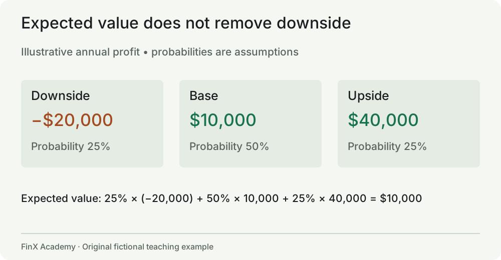
A positive expected value does not eliminate the possibility of loss. A company may lack the liquidity to survive the downside, or the assumed probabilities may be poorly supported. Expected value is a summary of the stated distribution, not an instruction to take every positive-average gamble.

Check that probabilities are nonnegative and sum to one, and that the scenarios are mutually exclusive and collectively cover the modeled possibilities. If your scenarios are simply illustrative stress tests, label them that way instead of inventing probability weights.

Do not substitute average inputs blindly

If profit = 12 × units − 36,000 with fixed coefficients, applying the formula to expected units gives expected profit because the relationship is linear. That shortcut can fail when the model includes thresholds, capacity steps or nonlinear relationships. For example, the average of two growth rates applied twice is not generally the average of the two compounded outcomes.

Model each relevant scenario, then weight its output. Also think about joint behavior: high demand may cause overtime costs, while a higher price may reduce volume. Treating related inputs as independent can produce implausible combinations.

Correlation describes co-movement, not a cause

Suppose hot weather increases both cold-drink sales and bottled-water sales. The two sales series may move together without either causing the other. Seasonality is a common driver. A correlation coefficient summarizes linear association between −1 and +1; it does not identify the mechanism, prove causation or exclude a nonlinear relationship when near zero.

Before making a causal claim, inspect timing, plausible mechanisms, confounders, sample selection and alternative explanations. A carefully designed experiment or stronger research design can provide better evidence than a simple chart. Forecasting from an association also requires checking whether the relationship remains stable outside the sample.

Check yourself

1. For 2, 3, 4, 5 and 36, calculate the mean and median. Which better describes the middle observation?
2. A project returns −$50 with probability 20% and +$20 with probability 80%. What is its expected outcome? Can it still lose money?
3. A chart shows advertising and revenue rising together. Name two explanations besides “advertising caused all the revenue growth.”

Answers and reasoning

1. Mean 10; median 4. The median describes the middle position; the mean still correctly reproduces the total of 50.
2. +$6 = −50 × 0.20 + 20 × 0.80. The modeled loss probability remains 20%.
3. A seasonal peak could drive both; managers could increase advertising because revenue or expected demand is already rising. Product changes, prices and distribution could also contribute.

Transfer task: write a forecast sentence containing an amount, a horizon, the assumptions and one reason the outcome could differ. Then decide whether your evidence supports a point estimate, scenarios or probabilities.

9. Capstone: should Northstar expand?

Northstar’s manager says: “The expansion has a positive NPV in the base case, so let’s do it.” Your task is to check the arithmetic and test whether the conclusion follows. Work through the questions before opening the solution. A calculator is enough; the optional sandbox provides the same mechanics.

What you will submit: a small calculation table and a recommendation of 120–180 words. State the assumptions, distinguish operating profit from project cash flow, and explain which information would change your view.

The case pack

These are new, explicit capstone assumptions. Do not carry the optional capacity examples from earlier lessons into this case. All amounts are USD. Ignore tax, financing, inflation and depreciation effects here; these simplifications will be relaxed in later courses.

Without expansion, the line can make and sell 4,000 bottles each month. Price is $30, variable cost $18, and monthly fixed costs $36,000. That situation continues for the next two years. Demand beyond 4,000 cannot be served without expansion.

Expansion costs $60,000 today and requires another $12,000 of working capital today. Working capital here means cash committed to supporting operations; assume the full $12,000 is recovered at the end of Year 2 in every scenario. The equipment has no terminal value. Expansion raises capacity to 5,500 bottles/month and fixed costs to $42,000/month. Price and unit variable cost stay unchanged.

Incremental operating profit is assumed to convert one-for-one into incremental operating cash, apart from the separately stated initial investment and working-capital movements. Aggregate annual cash flows occur at each year-end. Demand is constant within each scenario for both years:

Scenario	Monthly units sold with expansion	Assumed probability
Downside	4,000	20%
Base	4,750	60%
Upside	5,250	20%

The required return is 8% effective annually. Probabilities are supplied teaching assumptions, not observed evidence. The relevant alternative is continuing without expansion, not shutting down the business.

Your analysis

1. Calculate the current monthly revenue, contribution and operating profit. Label the units and period.
2. Calculate the current contribution margin, markup over variable cost and break-even volume. Explain the denominators.
3. Calculate monthly operating profit with expansion in each scenario. Then calculate the incremental monthly result versus continuing without expansion.
4. Calculate the expansion’s break-even volume for zero total operating profit. Separately calculate the volume needed to match the existing $12,000 monthly profit. Why are these different?
5. Construct the base-case project timeline, including working capital. Calculate NPV and explain its meaning.
6. Calculate NPV for the downside and upside. Calculate probability-weighted NPV. Does a positive base-case NPV settle the decision?
7. If all base-case project inflows move back one year while the $72,000 outflow remains today, what happens to NPV? Assume operations and working-capital recovery shift together.
8. A consultant’s $5,000 nonrefundable study was paid last month. Where does it belong in today’s incremental comparison?
9. The manager says base-case unit sales increase “by 18.75 percentage points.” Correct that statement. Is the percentage increase a two-year CAGR?
10. Write your recommendation and identify at least three assumptions to investigate. Separate arithmetic certainty from business uncertainty.

Worked solution — calculations and decision

1–2. Current economics. Monthly revenue is 4,000 × $30 = $120,000. Variable cost is $72,000, contribution $48,000, and operating profit $12,000. Contribution margin is 48,000/120,000 = 40%; markup over variable cost is 48,000/72,000 = 66.67%. Break-even volume is 36,000/12 = 3,000 units/month.

3. Expansion outcomes. Each unit still contributes $12. Deduct the new $42,000 monthly fixed cost, then compare against the existing $12,000 profit:

Scenario	Monthly revenue	Monthly operating profit	Incremental profit/month	Incremental operating cash/year
Downside	$120,000	$6,000	−$6,000	−$72,000
Base	$142,500	$15,000	$3,000	$36,000
Upside	$157,500	$21,000	$9,000	$108,000

The downside business still earns positive operating profit. Its incremental project cash flow is negative because it performs worse than the alternative. That is not the same as saying the entire company’s cash flow is negative or that it must borrow this amount.

4. Two thresholds. Expanded-business break-even is 42,000/12 = 3,500 units/month. Matching the old profit requires (42,000 + 12,000)/12 = 4,500 units/month. The first threshold covers the expanded fixed-cost base; the second also preserves the profit of the alternative. Neither threshold alone recovers the upfront investment at a required return.

5. Base-case timeline. Today: −$72,000, comprising equipment and working capital. Year 1: +$36,000. Year 2: +$48,000, including $12,000 working-capital recovery. NPV = −72,000 + 36,000/1.08 + 48,000/1.08² = +$2,485.60. This is a modest modeled surplus over the required return, not $2,485.60 of guaranteed cash or annual profit.

6. Scenario values.

Scenario	Time zero	Year 1	Year 2 including working-capital recovery	NPV at 8%
Downside	−$72,000	−$72,000	−$60,000	−$190,107.00
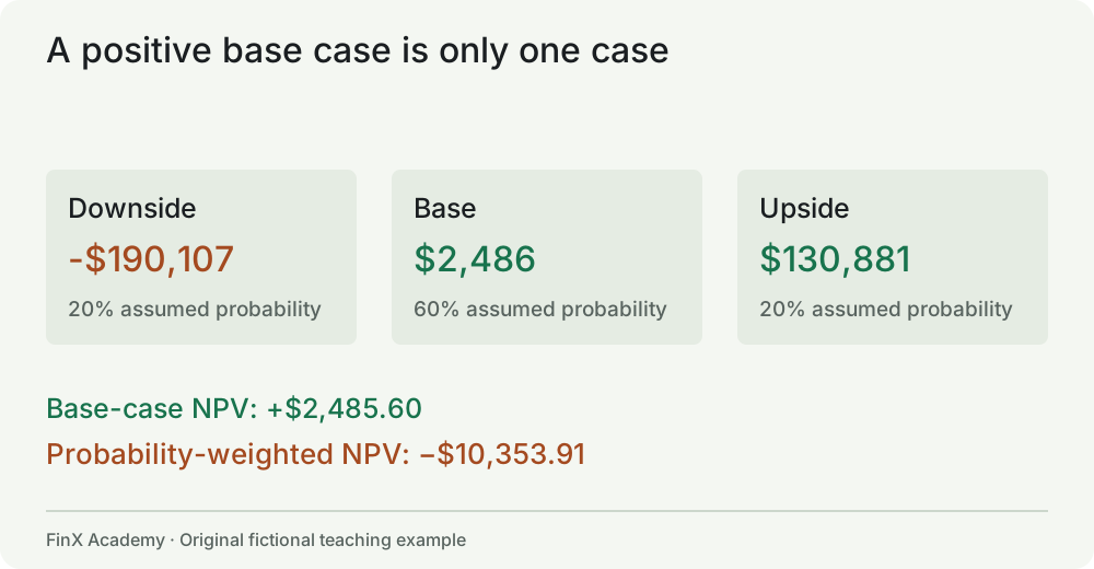
Base	−$72,000	$36,000	$48,000	$2,485.60
Upside	−$72,000	$108,000	$120,000	$130,880.66

Probability-weighted NPV is 20% × (−190,107.00) + 60% × 2,485.60 + 20% × 130,880.66 = −$10,353.91, using unrounded values internally. Equivalently, expected annual operating cash is $28,800; Year 2 also recovers $12,000. Discounting that expected timeline gives the same result because the dates and rate are common across scenarios. The base case being positive does not make the weighted case positive.

7. Delay. The timeline becomes −72,000 today, zero in Year 1, 36,000 in Year 2 and 48,000 in Year 3. NPV falls to −$3,031.85. Delayed benefits can reverse a thin positive case even if the undiscounted totals stay unchanged.

8–9. Decision hygiene. The nonrefundable study cost is sunk. Any further study cost caused by today’s decision is relevant. Unit volume rises (4,750 − 4,000)/4,000 = 18.75%, not percentage points. It is a change in the monthly run rate between alternatives, not a two-year compound growth trajectory.

10. Example recommendation. “Under the supplied assumptions, I would defer the expansion pending stronger evidence about demand and downside protection. The base case creates only $2,486 of value at an 8% required return, while the probability-weighted NPV is negative $10,354. A one-year delay also makes the base case negative. Expansion needs 4,500 monthly units simply to preserve current operating profit; that threshold does not recover the initial investment. I would investigate customer commitments supporting 4,750 units, whether the extra fixed costs can be reduced if demand disappoints, and whether working capital can really be recovered in full. The supplied probabilities are assumptions, so the weighted result is conditional. A staged or reversible expansion may improve the decision, but it needs its own cost and capacity model.”

Review your work

Award one point for each of the ten numbered tasks only when the calculation and explanation are consistent. For tasks 3 and 6, complete every scenario. A score is a self-check, not a credential. If you missed a timing item, revisit lessons 4–5; a denominator issue, lesson 2; an operating or counterfactual issue, lessons 6–7; or a probability interpretation, lesson 8.

For your recommendation, check four things: a clear decision, correct supporting numbers, explicit uncertainty, and a specific next investigation. A different recommendation can be reasonable if it acknowledges the same evidence and explains its decision criteria. It should not manufacture facts that are absent from the case.

Unseen variation: keep all other assumptions unchanged but replace the $60,000 equipment cost with $50,000. Predict the effect before calculating: every scenario NPV rises by exactly $10,000, because a time-zero payment changes dollar for dollar. The weighted NPV becomes −$353.91; the expected-value case is still slightly negative.

Review your recommendation

Use this rubric for self-review or a discussion with a tutor. It is a learning aid, not an automatically awarded certification. Give full credit only when the reasoning is shown; a copied final number is insufficient.

Evidence in your work	Points
Units, monthly/annual periods, scenario probabilities and the two-year horizon are explicit	3
Baseline and expanded operating profit reconcile; break-even and the old-profit threshold are distinguished	4
Incremental cash includes time-zero investment and one working-capital recovery; NPV timing is correct	5
Downside, weighted value and at least one decision-changing sensitivity are explained	4
Recommendation states its assumptions, a feasible alternative and the evidence that could change it	4

A useful readiness target is 16/20 with no unresolved cash-timing or incremental-cash error. Below that, revisit the corresponding lesson and solve a version with changed inputs. A numeric score does not replace the explanation: another person should be able to follow your comparison and identify its limits.

Further reading and how to use this course

The business, questions, diagrams and solutions in this course are original teaching examples. These references provide optional explanations of the underlying ideas; no textbook purchase is required, and the course does not reproduce their examples or worksheets.

• Time value: OpenStax, Time Value of Money Basics and Applications of TVM.
• Project return: OpenStax, Internal Rate of Return.
• Operating economics: OpenStax, Contribution Margin, Break-Even Analysis and Break-Even Sensitivity.
• Descriptive statistics: OpenStax, Measures of the Center of the Data.
• Relevant costs and pricing: OpenStax, Relevant Information for Decision-Making, Make or Buy a Component and Price Elasticity.

Download the text course or download the capstone inputs as CSV. The CSV contains assumptions, not a ready-made answer model. All answers are explained above.

For a second pass, choose one lesson you found difficult, explain it aloud without reading, and solve its check with changed numbers. Then continue into accounting and Excel foundations. Understanding the economic relationship first makes the spreadsheet easier to build and audit.