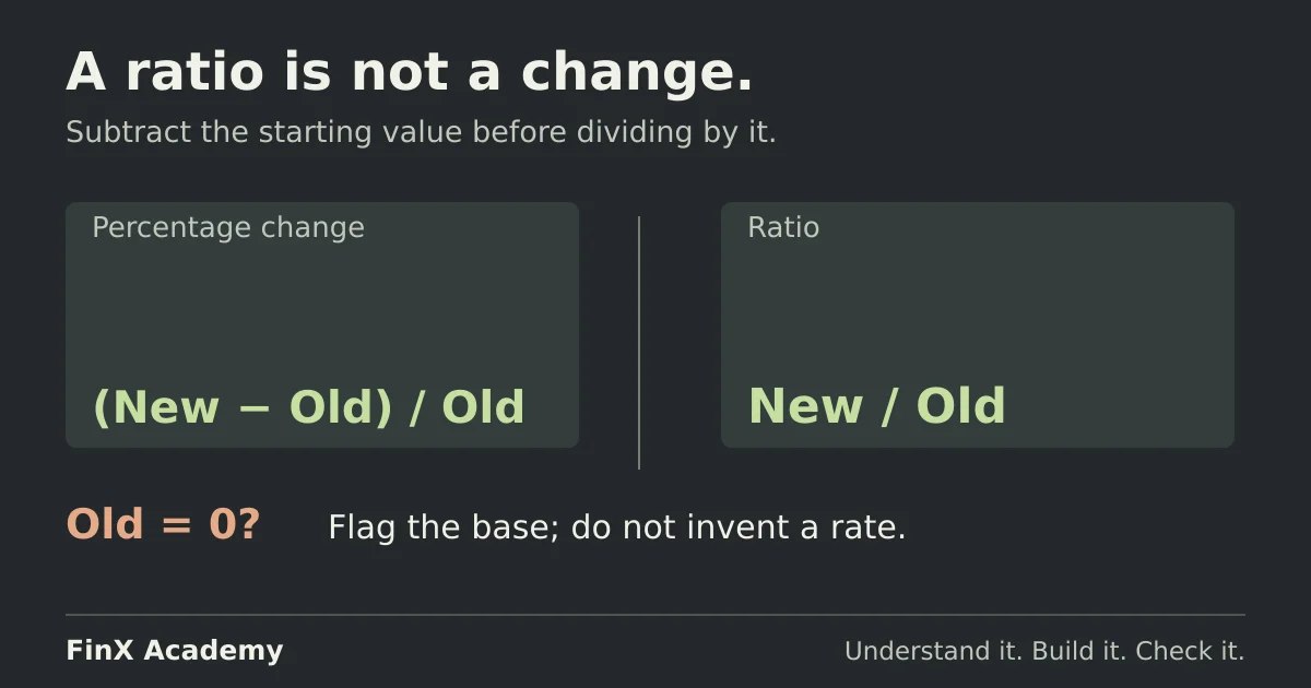
Percentage change in Excel: growth, declines and zero bases

One formula covers growth and decline in Excel:

=(C4-B4)/B4

Subtract the earlier value, divide by the earlier value, and format the cell as a percentage. Microsoft’s Calculate percentages page documents this difference-over-original calculation for both increases and decreases. The denominator is the whole question: percentage change always asks “change relative to what?”, and the answer is what you started with.

Three cases need extra explanation in a finance variance table: a zero base makes the division undefined; a negative base reverses the usual sign interpretation; and values that are already percentages allow both a percentage-point change and a relative percentage change. The worked example below covers all three.

Build the change table

Enter the headers in A3:E3 and this fictional quarterly comparison in rows 4–8 — all values in one set of illustrative units, the same quarter in the prior year versus the current year. The write-down amounts are negative because they are charges; the rest are positive.

Row	A: Item	B: Prior	C: Current	D: Change	E: % change
4	Revenue	250	300
5	Gross profit	100	135
6	Advertising	80	64
7	Asset write-down	−40	−25
8	New product line	0	30

Before typing anything, predict the first row by mental arithmetic: 250 to 300 is +50, and 50 is a fifth of 250, so +20%. Now enter in D4 and E4 and copy both down to row 8:

=C4-B4
=(C4-B4)/B4

Format column E as a percentage (Percent Style on the Home tab, two decimal places). A positive result need not display a plus sign unless you apply a custom number format; the plus signs below describe direction. The answers: revenue +20.0%, gross profit +35.0% (35 on a base of 100), advertising −20.0% (a 16 cut on 80). Then rows 7 and 8 stop looking like numbers you want in a report: the write-down shows −37.5% and the new product line shows #DIV/0!. Those two cells are the difference between a formula you type and a ratio you can defend.

The mistake that reports 120% instead of 20%

A very common shape of this formula drops the subtraction:

=C4/B4

With Percent Style this shows 120% for revenue — a reader who knows the growth was 20% spots the wrong number instantly, and a reader who doesn’t takes away the wrong story: ratios near 100% mean “no change”, but nothing on screen says the subtraction went missing. The ratio is not wrong as arithmetic; it answers a different question: “current as a percentage of prior”. The change is the ratio minus one: 1.2 − 1 = +20%. The tell is structural: with =new/old, an unchanged value shows as 100%, not 0%. Rebuild E4 as =(C4-B4)/B4 — or equivalently =C4/B4-1, which some analysts prefer because it mirrors the phrase “growth factor minus one” — and copy down; advertising now reads −20.0%, not 80.0%.

When the base is negative, the sign belongs to the base

Row 7 is the trap. The write-down improved: the charge fell from −40 to −25, so the loss shrank by 15, and D7 correctly shows +15. But E7 divides by the prior value −40 and prints −37.5%, which reads as a deterioration. The magnitude is genuine — the loss did shrink by 15/40 = 37.5% of its old size — while the sign is an artifact of dividing a positive improvement by a negative base.

For this report, when the base is negative, show the change in units and describe the direction in words — “write-down narrowed from 40 to 25” — rather than treating the percentage sign alone as favourable or unfavourable. A positive base that crosses into a negative current value can still have an interpretable signed change: 40 to −10 is −125%, and should be labelled as a move from profit to loss. This is related to the reasoning the CAGR guide applies to multi-year series with negative endpoints: a ratio built on the wrong kind of base is not a measurement problem but a meaning problem.

When the base is zero, guard the division

Row 8 grew from no prior-year revenue to 30. Division by zero has no answer: Microsoft’s #DIV/0! correction page documents division by zero, including a zero or blank denominator cell, and shows how to test the denominator before dividing. Applying that pattern here: =IF(B8=0,"n.m.",(C8-B8)/B8). This is our example formula; Microsoft uses different cells and output text. With the guard, E8 reads n.m. — not meaningful — and the honest statement is the absolute one: +30 from a standing start.

Keep two reporting issues in view:

• An IFERROR wrapper (=IFERROR((C8-B8)/B8,"n.m.")) is tempting but is a blanket handler — it can hide other formula errors, including a broken reference you wanted to catch. Test the denominator, not any error.
• The guard’s output is text. AVERAGE ignores text in a referenced range, so =AVERAGE(E4:E8) can omit a flagged row silently. Keep the source values and flags visible. Revenue, gross profit and expenses in this table are different measures; summing them would double count or mix concepts, so do not calculate a total growth rate for this table.

Percentage points or percentage change? A margin makes both

Gross margin is already in this table: =B5/B4 is 40.0% last year, =C5/C4 is 45.0% this year. Someone asks: “how much did margin improve?”

• Percentage-point change — the move on the percentage scale: 45.0 − 40.0 = 5.0 points.
• Percentage change — the relative move: (45 − 40)/40 = +12.5%.

Both are correct answers to different questions, and Excel will hide the distinction if you let it: subtracting two percentage-formatted cells (0.45 − 0.40) gives 0.05, which Percent Style renders as a suspicious-looking “5.00%” that is really 5 percentage points. Say which one you mean.

Then reconcile with row 5, because the same table proves the result from another direction: gross profit grew +35% against revenue’s +20%, and 1.35 ÷ 1.20 − 1 = 12.5% — the profit line outgrew the sales line by exactly the margin’s relative improvement. Two computations, one fact. The Excel for finance budget report shows the related aggregation rule up a level: divide the total difference by the total budget rather than averaging a column of percentages.

Choose the next practice step

Type the formula once as (new − old)/old, check it by predicting the row you can do in your head, guard the denominator instead of wrapping errors, and switch to absolute change and words whenever a base is negative or zero.

For a multi-year growth story built on the same instinct, the CAGR guide compounds percentage changes and catches the off-by-one period count; for when a fixed denominator needs an anchor, see the absolute-reference guide. Here the denominator must move from B4 to B5 as you copy down, so keep it relative; and the Excel for finance learning guide places the variance column inside a report you can reconcile to its source.

In FinX’s Excel for Finance course, Mathematical Functions and Anchoring & the Grid are free; later lessons that build on these mechanics require paid access. Browse the catalogue for current syllabus and pricing, or try the free five-question diagnostic to find the skill to practise next.