Excel for finance: learn the skills by building a budget report

Start learning Excel for finance with a small report whose answer you can check. You should be able to identify its inputs, select the right records, copy its formulas and explain the difference between the result and the plan.

The January expense report below totals 3,700 against a budget of 3,700. That looks reassuring until you inspect the departments: Sales is 200 over budget, while Operations and Support are each 100 under. Building and checking this report connects several useful skills without requiring a full valuation model.

Learn the skills in a useful sequence

You can start this exercise once you can enter numbers, select cells and write a basic arithmetic formula. Build from there:

Stage	Skill to practise	Evidence that it works
1. Build the calculation	Arithmetic, SUM and relative/absolute references	The first formula and its last copied cell both use the intended inputs
2. Prepare the source	Consistent labels, numeric amounts and explicit periods	You can explain what each row represents and identify missing or duplicate records
3. Retrieve and summarise	Lookups for attributes; SUMIFS for conditional totals	You can distinguish returning one match from adding all matching records
4. Explain the output	Variances, assumptions and reconciliation	You can trace a difference back to its cause
5. Extend the model	Scenarios, sensitivity and financial functions	Changing an assumption affects the expected outputs, with its meaning preserved

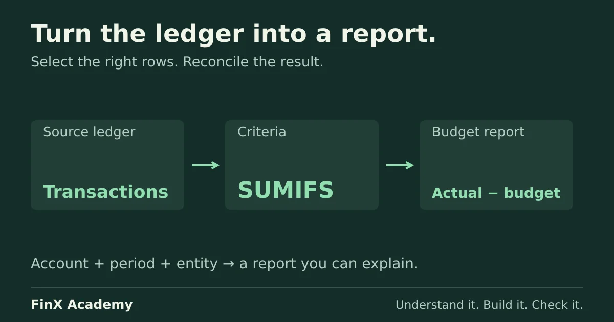
Use the absolute-reference guide if copied formulas move away from their assumptions. The XLOOKUP practice teaches matching records and inspecting missing or duplicate keys. The exercise here adds conditional aggregation: several expense records belong in each departmental total. The SUMIF vs SUMIFS guide compares the two functions and covers date-boundary criteria on an invoice ledger. If a total ignores rows because amounts arrived as text, the convert text to numbers guide diagnoses the silent undercount and repairs it without damaging account codes.

Set up a small expense source

Use a blank worksheet. All figures are fictional expenses in one currency, entered as positive costs. Every record belongs to one illustrative year; numeric month codes 1 and 2 mean January and February.

Put the reporting month in B1 as 1. Enter these headers in A3:C3 and records in rows 4–11:

Row	A: Month	B: Department	C: Expense
4	1	Sales	1,200
5	1	Sales	800
6	1	Operations	700
7	1	Operations	500
8	1	Support	300
9	1	Support	200
10	2	Sales	900
11	2	Support	400

Enter amounts as numbers, using formatting for separators or currency symbols. Keep labels consistent and preserve the source rows so you can trace a total back to its components. These repeated department names represent different expense records, not duplicate transactions.

The two-month source makes a period-selection mistake visible. In a real file covering several years, use a full period identifier or date range so January from different years cannot be combined accidentally.

Summarise the right month and department

Create the report headers in E3:I3. Enter department names in E4:E6 and the January budgets in F4:F6. The remaining columns are calculated:

Department	Budget	Actual	Actual − budget	Variance %
Sales	1,800	2,000	200	11.11%
Operations	1,300	1,200	−100	−7.69%
Support	600	500	−100	−16.67%

In G4, enter:

=SUMIFS($C$4:$C$11,$A$4:$A$11,$B$1,$B$4:$B$11,E4)

Copy down to G6. The formula adds expenses only when both conditions match: the month equals B1 and the department equals the label in column E.

The amount range comes first in SUMIFS, followed by pairs of criteria ranges and criteria. Each range here covers the same eight source rows. See Microsoft’s SUMIFS documentation for the argument order and range requirements.

The dollar signs hold the source ranges and reporting month fixed. The department reference moves from E4 to E5 and E6. In the last copied formula, it should still read $B$1 for the month and E6 for Support. Microsoft’s reference guide explains this copy behaviour.

A lookup returning one Sales expense would not answer this question: January has two Sales records, and both belong in the total.

Calculate variance with a clear sign convention

In H4, enter =G4-F4. In I4, enter =H4/F4. Copy both formulas down to row 6 and format column I as a percentage with two decimal places.

We use actual minus budget for positive expense amounts. A positive variance means overspending; a negative variance means underspending relative to this plan. Whether lower spending is operationally desirable still needs explanation.

All budgets in this example are positive. If a budget is zero, its percentage variance is undefined; show that limitation explicitly instead of turning a division error into a false 0%. The percentage change guide works through exactly that case, plus negative bases and the percentage-point distinction.

Put Total in E7, then use =SUM(F4:F6) in F7, =SUM(G4:G6) in G7, =G7-F7 in H7 and =H7/F7 in I7. Both totals are 3,700, so the overall variance is zero.

Do not average the three departmental variance percentages to calculate the total. Divide the total difference by the total budget. The zero overall variance here contains offsetting departmental differences; it does not mean each department met its plan.

Reconcile the report to its source

Build a separate check below the source:

Cell	Calculation	Formula	Answer
B14	All source expenses for the selected month	=SUMIFS($C$4:$C$11,$A$4:$A$11,$B$1)	3,700
B15	Expenses included in the departmental report	=SUM(G4:G6)	3,700
B16	Report minus source	=B15-B14	0

This check asks a different question from budget variance: did the report include the selected month’s source expenses? The source total does not depend on the report’s department list, so it can expose omitted categories or incorrect departmental formulas.

It cannot prove the source itself is correct. Duplicate transactions, wrong amounts or offsetting errors may still pass. For this small example, also add January’s six entries manually: 1,200 + 800 + 700 + 500 + 300 + 200 = 3,700.

Remove one condition and follow the error

Temporarily replace G4 with this formula and copy it down to G6:

=SUMIFS($C$4:$C$11,$B$4:$B$11,E4)

The month condition has disappeared. Sales becomes 2,900, Operations stays 1,200, and Support becomes 900. The report now totals 5,000, including February’s 1,300 of expenses.

The source check in B14 still selects January. The reconciliation difference in B16 therefore becomes 1,300, directing you to the selection logic instead of suggesting a change to the budget.

Restore the original two-condition formula and copy it down. Then increase the second January Sales expense in C5 from 800 to 900. Sales actual should become 2,100, total actual 3,800, and total budget variance 100. The source reconciliation should remain zero, because both source and report reflect the same change. Restore C5 to 800 afterwards.

The fixed source range ends at row 11. Appending records below it requires expanding every relevant range or adopting a controlled expanding table; a formula that ignores new rows will not repair itself.

Choose the next practice step

If this report was difficult, identify the specific gap. Practise references if copying broke it, data preparation if labels or amounts failed to match, and conditional aggregation if the wrong records entered the total. Once it works, the sensitivity-analysis guide shows how to vary assumptions and compare outputs.

FinX’s Excel for Finance course follows these areas through foundations, lookups, aggregation and data hygiene, model mechanics, and financial functions. Mathematical Functions and Anchoring & the Grid are free; the later lessons, including XLOOKUP and Conditional Aggregation, require paid access. Browse the catalogue for the current syllabus and access details.

For planning version control, work through budget vs forecast. Before aggregating a payment extract, review duplicate records without deleting legitimate transactions.