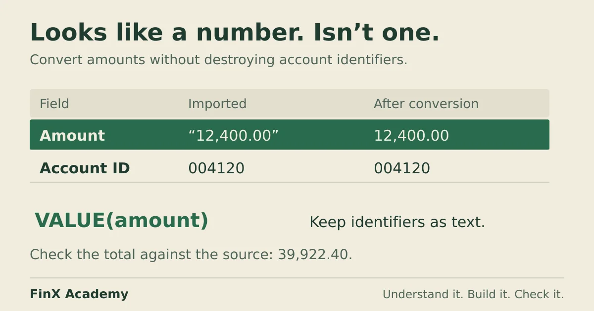
Convert only the amount column and reconcile the result to a source control total. SUM ignores text-stored amounts without an error, and converting an identifier column silently deletes its leading zeros.
When an import lands amounts as text, SUM quietly skips those rows: Microsoft’s
SUM documentation
states that SUM “will ignore text values and give you the sum of just the numeric values.” You get a
wrong total with no error to find. The repair is to convert the amount column and reconcile the
result to a figure from the source — but convert only that column. The same conversion applied to
an account-code column destroys leading zeros, and the damaged identifiers fail lookups silently
too.
Reproduce the broken import
Enter the headers in A3:C3 and the eight records in rows 4–11 of a blank worksheet. These are
fictional records in one currency, all positive. The Stored as column is instruction, not a header
to type: enter the four text amounts with a leading apostrophe — '12,400.00 — which forces Excel
to keep them as text. Enter the numeric amounts as plain numbers. This example assumes US separators:
a period for decimals and a comma for thousands. For a different source convention, use the explicit
separator conversion described below.
| Row | A: Account | B: Memo | C: Amount | Stored as |
|---|---|---|---|---|
| 4 | 004120 | Client invoice | 12,400.00 | text |
| 5 | 101230 | Client invoice | 3,250.75 | number |
| 6 | 004130 | Retainer | 980.50 | number |
| 7 | 101230 | Client invoice | 15,000.00 | text |
| 8 | 004120 | Reimbursement | 4,125.25 | number |
| 9 | 203400 | Subscription | 2,375.00 | text |
| 10 | 101230 | Client invoice | 1,150.00 | number |
| 11 | 203400 | Subscription | 640.90 | text |
Type the account codes as text too ('004120); the source system uses fixed six-character codes,
and that detail is the point of the failure case below. Suppose the export carries a control total —
a footer line or the covering email — reading 39,922.40.
Diagnose the total that skipped rows
Put Ledger total in E4 and enter in F4:
=SUM(C4:C11)The answer is 9,506.50, not 39,922.40. Nothing is red and no cell shows an error. Two checks
locate the problem. In E5/F5 put Counted with =COUNT(C4:C11), and in E6/F6
Non-empty with =COUNTA(C4:C11). You get 4 and 8: only four of the eight amounts are
numbers, and SUM added exactly those. Microsoft’s
conversion guide
describes the visual tells — text is left-aligned by default while stored numbers are right-aligned,
and text-stored numbers often carry the small green error indicator in the corner.
The four skipped rows are 12,400.00 + 15,000.00 + 2,375.00 + 640.90 = 30,415.90, and
9,506.50 + 30,415.90 = 39,922.40 — the control total, exactly. The diagnosis is complete before
any repair: every missing cent is accounted for.
Convert only the amount column
Choose one of these documented routes for C4:C11, using the stated separator convention. All eight
amounts should then be numbers; verify the count and total before proceeding.
- Convert to Number. Select
C4:C11, open the error indicator on any selected cell and choose Convert to Number. This route is available when Excel exposes the number-stored-as-text error action. If error checking is disabled or the action is unavailable, use another method below. - Paste Special, multiply by 1. Type
1in an empty cell and copy it. SelectC4:C11, open Paste Special and choose Multiply. Microsoft’s troubleshooting article explains why it works: multiplying each cell by 1 replaces the text with its numerical equivalent, so the display barely changes but the stored type does. - A
VALUEhelper column. InE8enter=VALUE(C4), fill down throughE15, then copy those eight results overC4:C11with Paste Special > Values, as the conversion guide instructs.VALUEconverts “text that represents a number” and returns#VALUE!on anything not in a recognised format, so the conversion itself reports which rows it could not read.
Changing the number format dropdown alone does not parse existing text amounts into numbers. Likewise, formatting already-damaged identifiers as Text does not recover digits that were removed. Microsoft’s leading-zeros article explains why the intended storage type should be set before entry.
Confirm F4 now reads 39,922.40 and =COUNT(C4:C11) reads 8. Then reconcile per account,
which is the check that the conversion matched each row to the right record and not just added up:
| Account | Rows | Total |
|---|---|---|
| 004120 | 12,400.00 + 4,125.25 | 16,525.25 |
| 004130 | 980.50 | 980.50 |
| 101230 | 3,250.75 + 15,000.00 + 1,150.00 | 19,400.75 |
| 203400 | 2,375.00 + 640.90 | 3,015.90 |
| All | 39,922.40 |
The mistake that damages identifiers
On a copy of the practice sheet, apply Paste Special > Multiply by 1 to A4:A11, the identifier
column, after repairing the amounts. F4 still reads 39,922.40, so the report looks healthy. But the account
codes were number-shaped text too, and Excel converted 004120 to the number 4120: its
documentation
says leading zeros are removed automatically, with account numbers among the examples.
The damage surfaces in a lookup. To reproduce it in an Excel edition with XLOOKUP, enter '004120
in H4 and Client income in I4, representing one chart-of-accounts record. Then enter:
=XLOOKUP(A4,$H$4:$H$4,$I$4:$I$4,"Check account")The converted numeric 4120 in A4 no longer matches the original text 004120 in H4, so the
result is Check account. =LEN(A4) returns 4 instead of 6. Exact lookups depend on compatible
keys; do not assume every Excel function uses the same text/number coercion rules.
One repair and one prevention:
- Repair the fixed-width codes. With a six-character standard,
=TEXT(A4,"000000")rebuilds004120as text — the same route as Microsoft’s postal-code example. Build the corrected codes in a helper column, then paste them back as values into a Text-formatted account column. The lookup should now return Client income. This works only because the format is known and fixed-width: Excel keeps 15 significant digits, so a code whose lost digits sat beyond the fifteenth cannot be recovered and must be kept as text from entry onwards. - Prevent it. Convert one column at a time —
C4:C11, not the block — and give the account column the type it should always have had: format it as Text before typing or pasting, or keep the apostrophe prefix.
The general lesson: a conversion that turns an identifier column into numbers can pass every total check on the sheet while breaking every join that depends on the identifiers. Reconcile what you convert against what references it.
When conversion fails: stray spaces and foreign formats
Two cases need closer inspection before choosing a conversion:
- Hidden characters. Do not assume an ordinary leading or trailing space necessarily causes a
conversion error. Inspect the actual character. Microsoft’s TRIM reference
notes that TRIM handles ordinary ASCII spaces but not the nonbreaking space numbered 160.
CLEAN removes the first 32 ASCII
control characters, not every Unicode character. For a known nonbreaking-space import, a helper such
as
=VALUE(TRIM(CLEAN(SUBSTITUTE(C4,CHAR(160)," "))))replaces that character before conversion. Reconcile afterwards; this is not a universal cleanup rule for every source format. - Separator styles. A branch file may send
1.250,40— European style, thousands point and decimal comma. In an English (US) workbook that is not a recognised format, soVALUE("1.250,40")returns#VALUE!. The NUMBERVALUE function is documented as locale-independent and takes the separators as arguments:=NUMBERVALUE(C4, ",", ".")reads1.250,40as 1,250.40. Check which separators your system setting uses before assuming either order.
Choose the next practice step
Diagnose with COUNT against COUNTA and a source control total; convert only the amount column;
keep identifiers as text before entry, not after; and reconcile the converted report per account so
the totals and the joins are both checked.
Aggregating the cleaned ledger is the next skill: the SUMIF vs SUMIFS guide builds checked conditional totals on an invoice ledger, and the Excel-for-finance learning guide places both in a full spreadsheet sequence. If damaged keys are the recurring problem in your real work, the VLOOKUP practice exercises drill match failures including an identifier stored as text.
In FinX’s Excel for Finance course, Mathematical Functions and Anchoring & the Grid are
free; the Cleaning Analyst Data lesson, which drills TRIM/CLEAN work on an export, requires
paid access. Browse the catalogue for current syllabus and pricing, or try the
free five-question diagnostic to find the skill to practise next.
When cleaning an extract, the remove duplicates guide shows why normalized identifiers still need an independent payment-register check.
Continue with guided practice
Build on this guide with spreadsheet exercises on formulas, lookups and financial functions. Explore the syllabus and start with a free lesson.
Excel for Finance course