VLOOKUP practice: three finance exercises with worked answers

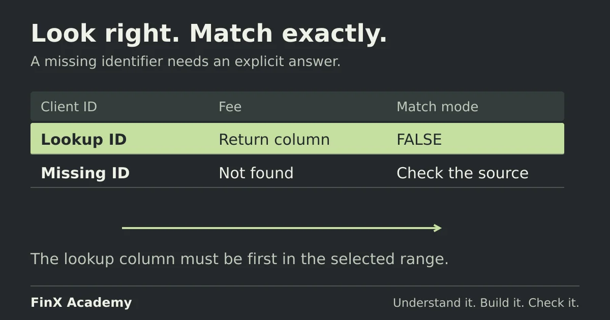
VLOOKUP searches down the first column of a range and returns a value from a column to its right. It is available in every Excel version from 2016 to current Microsoft 365, so it still appears in shared workbooks, tests and handovers even where XLOOKUP would be the better choice. If you are deciding which function to use rather than practising this one, read the XLOOKUP vs INDEX MATCH comparison first.

These three exercises use one small fictional dataset: a client rate card and an invoice ledger. Each exercise has a worked answer and a realistic failure to diagnose. Everything can be typed into a blank worksheet in a few minutes; there is no file to download. Microsoft’s VLOOKUP documentation is the reference for the behaviour discussed here.

Set up the practice data

Enter this fictional rate card in A1:C7. The Row column below identifies worksheet rows; do not enter it as data. Client IDs are numeric and sorted ascending, which matters in exercise 1. Enter rates as plain numbers such as 1.8, not as 1.8%; the fee formula later divides by 100.

Row	A: Client ID	B: Client	C: Fee rate %
2	101	Ashford Capital	1.8
3	104	Bridle Lane Fund	2.1
4	107	Cedar Hill Trust	1.5
5	112	Danforth Partners	2.4
6	118	Eastgate Holdings	1.2
7	125	Fairmont Estates	2.0

Then enter a rebate tier table in A10:B14: headers in row 10, volume thresholds in column A and rebate rates as plain numbers in column B. Rows 11–14 are 0 → 0, 25,000 → 0.5, 60,000 → 1.0 and 120,000 → 1.5.

Finally, enter an invoice ledger in G1:I7 with headers Invoice, Client ID and Billable amount:

Invoice	Client ID	Billable amount
INV-2001	101	40,000
INV-2002	107	25,000
INV-2003	112	60,000
INV-2004	118	30,000
INV-2005	104	55,000
INV-2006	101	20,000

Amounts are illustrative units. Client 101 appears twice: two invoices for the same client are normal in a ledger, and the rate card holds one record per client.

Exercise 1: choose the match mode on purpose

Put a client ID in E2 — start with 107 — and this formula in F2:

=VLOOKUP(E2,$A$2:$C$7,3,FALSE)

The four arguments are: the value to find, the table range, the column number to return from (counting from the table’s leftmost column), and the match mode. FALSE requests an exact match. Answer: 1.5, Cedar Hill Trust’s rate.

Now delete the fourth argument and look up an ID that does not exist. With E2 = 110:

=VLOOKUP(E2,$A$2:$C$7,3)

Answer: 1.5 — and it is wrong. The omitted argument defaults to approximate match, which finds the closest value not greater than 110: client 107. A nonexistent client silently receives Cedar Hill’s rate. The same formula with ,FALSE returns #N/A, which is the honest answer: no such client.

Approximate match is not a defect; it is the right tool for tiered data. With an amount of 78,000 in E5:

=VLOOKUP(E5,$A$11:$B$14,2,TRUE)

Answer: 1.0. The lookup finds the largest threshold at or below 78,000, which is 60,000. That works only because column A is sorted ascending — Microsoft’s documentation warns that with TRUE or an omitted argument, an unsorted first column can return a value you do not expect. Tier lookup wants approximate match; identifier lookup wants FALSE. Decide which one the column holds.

Exercise 2: copy the formula down the ledger

Label J1 “Fee rate %” and K1 “Fee”. In J2, a colleague has written the formula without dollar signs:

=VLOOKUP(H2,A2:C7,3,FALSE)

J2 returns 1.8, and filling the formula down to J7 appears to work: rows 2 to 5 return 1.8, 1.5, 2.4 and 1.2.

The last two rows are broken. Because the table range is relative, each copied row slides it down by one: J6 searches A6:C11 and J7 searches A7:C12. Client 104 in row 6 and client 101 in row 7 fall outside the shrunken lookup column, and both return #N/A. The first rows look correct, which is exactly why this survives a quick glance.

The fix is to lock the table range:

=VLOOKUP(H2,$A$2:$C$7,3,FALSE)

Filled down, the six answers are 1.8, 1.5, 2.4, 1.2, 2.1 and 1.8. Then compute the fee in K2 as =I2*J2/100 and fill down:

Invoice	Fee rate %	Fee
INV-2001	1.8	720
INV-2002	1.5	375
INV-2003	2.4	1,440
INV-2004	1.2	360
INV-2005	2.1	1,155
INV-2006	1.8	360

Answer: total fees of 4,410 (=SUM(K2:K7)). As a control total, it should also equal the sum you get by re-rating each invoice independently.

Two related failures to try while you are here:

• Change the column number to 4 in J2. The table has three columns, so VLOOKUP returns #REF!. The column index counts from the table’s leftmost column, not from column A of the sheet.
• Replace $A$2:$C$7 with A2:B7 and keep the index 3. #REF! again: the return column must be inside the range you pass.

The absolute-reference guide explains which parts of a range should move when a formula is copied.

Before the next exercise, restore J2 to =VLOOKUP(H2,$A$2:$C$7,3,FALSE) and fill it through J7. Confirm that the existing fee formulas in K2:K7 again total 4,410.

Exercise 3: handle the missing identifier

Add a seventh invoice in G8:I8: INV-2007, client ID 130, amount 45,000. Enter the locked exact-match formula in J8:

=VLOOKUP(H8,$A$2:$C$7,3,FALSE)

Answer: #N/A. Client 130 is not on the rate card. With the fourth argument omitted, the same lookup returns 2.0 — Fairmont’s rate, because 125 is the closest ID below 130 — and the ledger would bill a 900 fee that belongs to nobody.

Make the missing record visible instead of numeric:

=IFNA(VLOOKUP(H8,$A$2:$C$7,3,FALSE),"Check rate card")

Do not default the gap to 0. A client with a genuinely negotiated zero rate and a client missing from the rate card are different situations, and only the first should produce a zero fee. Keep this invoice’s fee unresolved until its rate is confirmed; a total that excludes the unresolved invoice is not a complete billing total.

Before concluding that an identifier is truly missing, check its data type. Enter '118 in H8 to force text storage: an exact-match lookup against the numeric IDs returns #N/A even though 118 is in the table. Microsoft’s guidance warns about inconsistent storage types. Check =ISTEXT(H8) and =ISNUMBER(A6); both return TRUE in this mismatch. Alignment alone is not proof because formatting can change it. For this numeric-ID system, restore a numeric 118 to recover the 1.2 rate; systems with meaningful leading zeros should instead preserve text IDs on both sides.

Check your answers

• Client 107, exact match: 1.5.
• Client 110 with the argument omitted: 1.5 (wrong client); with FALSE: #N/A.
• Rebate tier for 78,000, approximate match on the sorted table: 1.0.
• Relative fill-down: rows 2–5 plausible, rows 6–7 #N/A; locked range: 1.8, 1.5, 2.4, 1.2, 2.1, 1.8 and total fees 4,410.
• Column index 4 on a three-column table: #REF!.
• Client 130: #N/A with FALSE, 2.0 with the default — and the text ID "118" also returns #N/A against numeric records.

Take the next practice step

The same failure modes exist in XLOOKUP, with one important difference: XLOOKUP defaults to exact matching, so the omitted-argument trap of exercise 1 does not arise in the same form. The open XLOOKUP practice exercises work through exact matches, missing departments and repeated records; FinX’s full XLOOKUP lesson is in the paid Excel curriculum, and the course catalogue shows its current access requirements. When one key column is not enough and the answer needs entity and account and date together, continue with the INDEX MATCH with multiple criteria exercises.

For a different kind of check, the free ten-minute diagnostic asks five numeric modelling questions. It is not a VLOOKUP assessment and does not grade this workbook.