XLOOKUP vs INDEX MATCH: choose and check your budget lookup

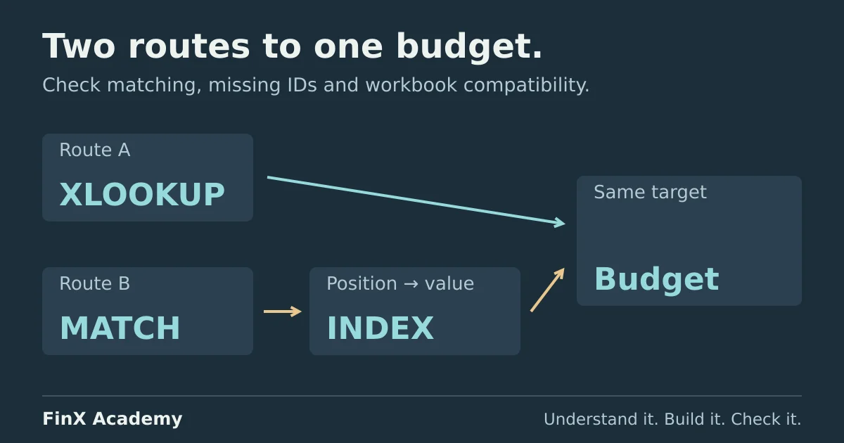
Use XLOOKUP for a straightforward lookup when everyone using the workbook has a version of Excel that supports it. Its exact-match default and built-in missing-value argument make the formula easier to read. Use INDEX with MATCH when the workbook needs compatibility with Excel 2016 or 2019, or when you are maintaining an existing model that uses that pattern.

Both can retrieve the correct budget. The more useful question is whether the formula still behaves correctly when a department is missing or the reporting month changes. In the example below, an omitted MATCH argument returns 1,300 for a department that does not exist.

Compare the decisions that affect your workbook

Decision	XLOOKUP	INDEX with MATCH
Excel compatibility	Available in Microsoft 365, Excel 2021 and Excel 2024; unavailable in Excel 2016 and 2019	The examples here also work in Excel 2016 and 2019
Exact matching	Default; match_mode of 0 makes the choice explicit	Set MATCH’s third argument to 0; omitting it selects approximate matching
Missing ID	Can return a message through if_not_found	Exact MATCH returns #N/A when it cannot find the ID
Return a value to the left	Supported through a separate return range	Supported through a separate INDEX range
Department and month lookup	Nest one XLOOKUP inside another	Give INDEX a row MATCH and a column MATCH
Duplicate IDs	Default search returns the first match	Exact MATCH returns the first match

Microsoft’s XLOOKUP documentation explains its version availability, optional arguments and search direction. Its MATCH documentation explains the different default: 1, an approximate match that requires ascending data. The INDEX and MATCH guide demonstrates looking up values independently of the return column’s position.

For a new workbook on supported Excel versions, XLOOKUP is a useful starting choice. For an inherited model, understand and check its existing formulas before changing them. This small example is not a calculation-speed benchmark; measure a representative workbook if performance is the deciding factor.

Build one source table for both methods

Use a blank worksheet. These are fictional monthly department budgets in one currency, entered as positive numbers. There is exactly one row per department and one column per month. Enter the headers in A3:E3 and the data in rows 4–7:

Row	A: ID	B: Department	C: Jan	D: Feb	E: Mar
4	110	Sales	1,800	1,950	2,100
5	220	Operations	1,300	1,250	1,400
6	330	Support	600	650	700
7	440	Finance	900	950	1,000

Enter the month headers as the text Jan, Feb and Mar, not dates. Enter the IDs and amounts as numbers. Put Department ID in G2 and 220 in H2; put Month in G3 and Feb in H3.

The first task deliberately ignores the month selector: retrieve the January budget for ID 220. Find the answer in the source before entering a formula. It is 1,300, from Operations in row 5.

Retrieve January’s budget with each formula

Put XLOOKUP: Jan in G5 and this formula in H5:

=XLOOKUP($H$2,$A$4:$A$7,$C$4:$C$7,,0)

It searches the four IDs in column A and returns the aligned January value from column C. The empty fourth argument leaves the missing-value response as #N/A; the fifth argument, 0, explicitly requests an exact match.

Put INDEX MATCH: Jan in G6 and this formula in H6:

=INDEX($C$4:$C$7,MATCH($H$2,$A$4:$A$7,0))

Read this one from the inside out. MATCH returns 2 because 220 is the second item in A4:A7. INDEX then returns the second item in C4:C7: 1,300. The position is relative to the selected range, not worksheet row 2. See Microsoft’s INDEX syntax for how row and column positions select a result.

Both formulas should return 1,300. Their ID ranges and return ranges begin and end on the same source rows. Dollar signs hold these references fixed if you copy the formulas elsewhere; the absolute-reference guide explains which references to unlock when you build a report for several departments.

Test a missing ID before trusting the result

Change H2 to 230. That ID does not appear in the table. Both correct formulas should return #N/A, making the missing department visible.

Now temporarily remove the final ,0 from MATCH in H6:

=INDEX($C$4:$C$7,MATCH($H$2,$A$4:$A$7))

The result becomes 1,300. Because the IDs are sorted ascending, default approximate MATCH selects 220, the largest ID less than or equal to 230. INDEX faithfully returns that row’s January budget. The number looks reasonable but answers the wrong question.

This is a matching-rule error, not a reason to change the budget. Restore MATCH’s third argument to 0 and confirm the result becomes #N/A again. Exact matching does not require the IDs to be sorted; the sorted input here makes the approximate-match failure reproducible.

For a display cell, XLOOKUP can supply a clearer message:

=XLOOKUP($H$2,$A$4:$A$7,$C$4:$C$7,"Missing department",0)

With 230 selected, this returns Missing department. Do not use zero as the fallback unless a missing record truly means a zero budget in your process. A valid zero budget and an absent department are different conditions. Keep unresolved lookup errors visible before using the results in a total.

Restore H5 and H6 to their original exact-match formulas and reset H2 to 220 before continuing.

Select both the department and the month

The month selector in H3 now matters. With ID 220 and month Feb, the answer should be 1,250. Leave the January formulas in place so you can distinguish them from the new results.

Put XLOOKUP: selected month in G8 and enter in H8:

=XLOOKUP($H$2,$A$4:$A$7,XLOOKUP($H$3,$C$3:$E$3,$C$4:$E$7,,0),,0)

The inner XLOOKUP finds Feb in the month headers and returns that column’s four budgets: 1,950; 1,250; 650; 950. The outer XLOOKUP finds ID 220 and selects the corresponding value, 1,250. Microsoft’s XLOOKUP documentation includes this nested vertical-and-horizontal lookup pattern.

Put INDEX MATCH: selected month in G9 and enter in H9:

=INDEX($C$4:$E$7,MATCH($H$2,$A$4:$A$7,0),MATCH($H$3,$C$3:$E$3,0))

The first MATCH returns row position 2; the second returns column position 2. INDEX retrieves the intersection within C4:E7: 1,250. Both MATCH functions need 0 because both selectors identify a specific item.

Try these cases, reading the expected value from the source before checking the two formulas:

H2: ID	H3: Month	Expected H8 and H9
220	Feb	1,250
330	Mar	700
110	Jan	1,800
440	Feb	950
230	Feb	#N/A — missing department
220	Apr	#N/A — missing month

Reset the selectors to 220 / Feb, then change Operations’ February budget in D5 from 1,250 to 1,275. Both selected-month results should become 1,275. The January results should remain 1,300. Restore D5 afterwards.

Agreement between formulas is helpful, but it does not prove the input or the selected ranges are correct. Both formulas could be pointed at the same wrong source. Check the intended row and column as well.

Keep lookup rules separate from data problems

A department master with duplicate IDs needs investigation. The formulas here return the first matching row; neither automatically confirms that an ID is unique. XLOOKUP’s reverse-search option can select the last row, but “last in this range” only means “latest” if the source order establishes that meaning.

Likewise, a source containing several expense transactions per department needs aggregation when the question asks for total spending. Retrieving one record does not add the others. The Excel-for-finance budget report shows that separate task with SUMIFS and a source reconciliation.

When a valid-looking ID fails to match, check its value and data type in both places. A numeric ID and a text representation may need consistent preparation; Microsoft’s INDEX/MATCH error guide explains these missing-match checks. Preserve meaningful leading zeros in real identifiers rather than converting every code to a number. If you extend this example below row 7 or beyond March, expand the corresponding source ranges together.

The practical choice is the method your users can run, understand and test. Keep exact matching explicit for these IDs, make missing records visible, and verify a changed input. For more exercises, use the XLOOKUP practice with answers, which includes an optional browser sheet, or take the free five-question modeling test to identify a next skill to practise. When one lookup must satisfy several columns at once on older Excel, the INDEX MATCH with multiple criteria exercises work through duplicate combinations, missing matches and stored dates.