INDEX MATCH with multiple criteria: solve a finance lookup exercise

MATCH searches one row or column of values. When the answer lives at the crossing of three — entity, account and date — the classic pattern multiplies the conditions together and asks MATCH to find the first row where the product is 1:

=INDEX($E$2:$E$13,MATCH(1,($B$2:$B$13=H1)*($C$2:$C$13=H2)*($A$2:$A$13=H3),0))

Each comparison returns an array of TRUE/FALSE; multiplying turns them into 1s and 0s, and only a row satisfying every condition survives as a 1. The arithmetic is simple; the failure modes are where the practice pays. These three exercises use one fictional twelve-row expense ledger from the Tidewell group — Marina Retail (MRN), Quay South (QYS) and Pierpoint (PPA) — with a duplicate combination, a missing combination and a same-amount decoy built in. Amounts are illustrative units. Microsoft’s MATCH documentation covers the arguments; this page assumes you know single-criterion INDEX MATCH, or have read the XLOOKUP vs INDEX MATCH comparison — which is where the general “which function should I use” decision lives.

Set up the ledger and the criteria cells

Enter the headers in A1:E1 and the rows below in A2:E13. Enter column A as real dates (Excel keeps them as serial numbers; in the 1900 date system, 2026-02-02 is serial 46055) and the amounts as plain numbers.

Row	A: Date	B: Entity	C: Account	D: Ref	E: Amount
2	2026-01-12	MRN	Freight	FR-101	2,400
3	2026-01-12	MRN	Freight	FR-107	1,500
4	2026-01-12	QYS	Rent	RT-201	3,100
5	2026-01-19	MRN	Rent	RT-205	3,100
6	2026-01-19	QYS	Audit fees	AU-310	4,800
7	2026-01-26	PPA	IT	IT-402	900
8	2026-02-02	MRN	Freight	FR-118	2,100
9	2026-02-02	PPA	IT	IT-405	900
10	2026-02-09	QYS	Freight	FR-121	1,750
11	2026-02-16	MRN	Audit fees	AU-318	4,800
12	2026-02-16	MRN	Audit fees	AU-322	1,200
13	2026-02-23	PPA	Rent	RT-230	2,600

Put labels in G1:G3 (Entity, Account, Date) and the criteria in H1:H3: MRN, Freight, =DATE(2026,2,2). Use DATE(year,month,day) for the ledger dates too, and format them as dates. Note the criteria ranges: $A$2:$A$13, $B$2:$B$13, $C$2:$C$13 and the return range $E$2:$E$13 all begin and end on the same rows. Misaligned ranges are a class of wrong answer of their own; anchoring all four to rows 2–13 is part of the exercise.

Exercise 1: all three criteria, and a witness column

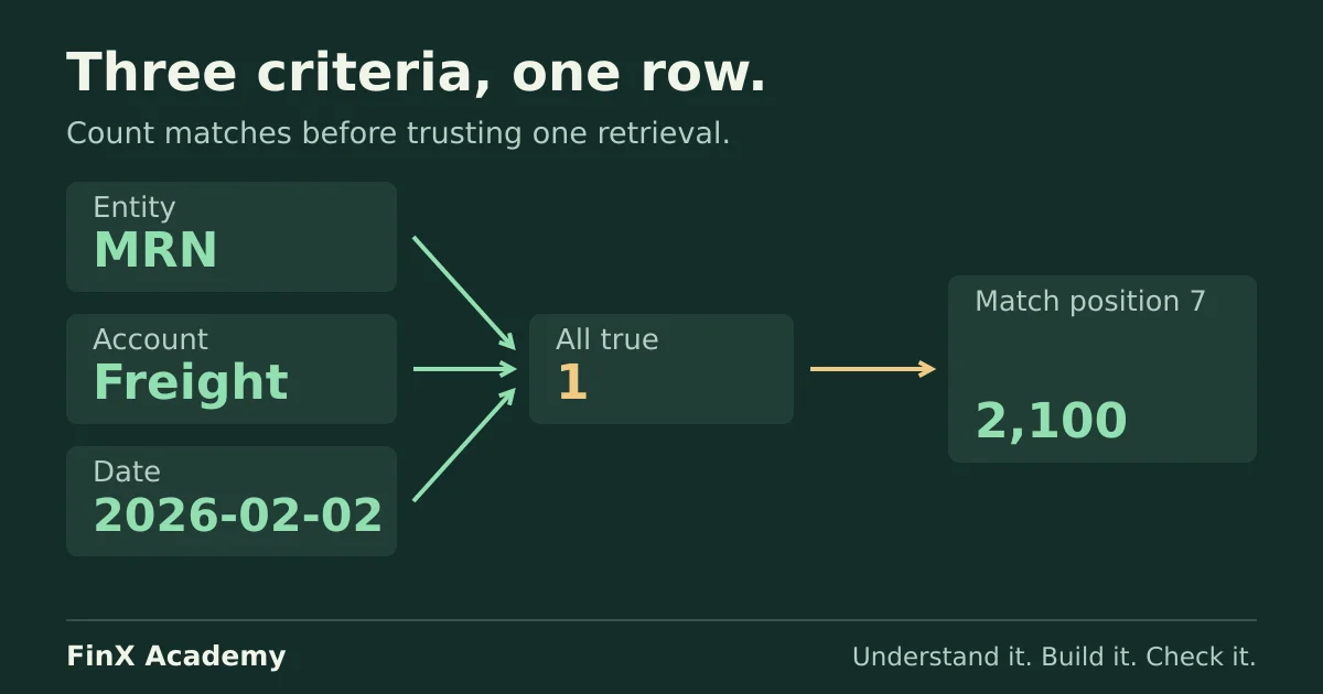
Enter the formula from the top of this page in H5. Answer: 2,100 — row 8, Marina Retail’s 2 February freight invoice. Inside MATCH, the product array is {0;0;0;0;0;0;1;0;0;0;0;0}: a single 1 in position 7, so MATCH returns 7 and INDEX returns the seventh value of E2:E13.

Incomplete or miswired criteria can return numbers anyway, which is what makes them dangerous:

• Drop the date condition and look up MRN freight: the product has a 1 at position 1, so the formula returns 2,400 — the January invoice, not the one you asked for.
• Swap two conditions — criteria QYS / Rent / 2026-01-19 matches nothing and says so (#N/A), but QYS / Rent / 2026-01-12 returns 3,100, and so does the MRN row on 2026-01-19. Rows 4 and 5 carry the same amount for different combinations. The amount cannot tell you which row was hit; the reference column can.

Retrieval is exactly why this pattern beats an aggregation here — it can return any column of the matched row. Copy the formula into H6 and change only the return range, $D$2:$D$13: FR-118. A formula whose witness cell returns RT-201 while you expected RT-205 has a condition wired to the wrong cell, and it will show up in the reference even when the amount matches by luck.

Exercise 2: duplicates, the count test, and the missing combination

Set the criteria to MRN / Freight / 2026-01-12. The lookup returns 2,400. Now add the two cells that turn that number into evidence:

Cell	Formula	Answer
H7	=COUNTIFS($B$2:$B$13,H1,$C$2:$C$13,H2,$A$2:$A$13,H3)	2
H8	=SUMIFS($E$2:$E$13,$B$2:$B$13,H1,$C$2:$C$13,H2,$A$2:$A$13,H3)	3,900

COUNTIFS returns 2 — two legitimate invoices were booked that day (FR-101 and FR-107; same-day duplicates are normal in ledgers, not dirty data). The retrieval answered with one of them: MATCH stops at the first 1. SUMIFS says the group spent 3,900; the difference, 1,500, is exactly the second invoice.

So decide the question before choosing the tool:

• “Which entry was it?” — retrieval, but only once COUNTIFS has returned 1. A first-match answer to a two-match question is a coin flip weighted by row order.
• “How much did it cost?” — aggregate: the same criteria pairs the SUMIFS guide drills; when every matching row counts, summing beats first-match.

Try the audit case: MRN / Audit fees / 2026-02-16 → retrieval 4,800, count 2, total 6,000, and the 1,200 difference is invoice AU-322. Then a genuinely absent combination, MRN / Audit fees / 2026-01-12: count 0, and the lookup returns #N/A. For a display cell:

=IFNA(INDEX($E$2:$E$13,MATCH(1,($B$2:$B$13=H1)*($C$2:$C$13=H2)*($A$2:$A$13=H3),0)),"no entry")

IFNA, not IFERROR: it turns only the honest no-match error into text, while a wiring bug like #REF! from a deleted source column stays visible. A source cell can itself contain #N/A, so confirm the count is zero before interpreting that error as an absent record. And “no entry” must not silently become zero downstream — an absent invoice and a zero-cost invoice are different facts.

Exercise 3: the date criterion is stored wrong, then the key route

Reset to MRN / Freight / 2026-02-02, which returns 2,100. Now replace the date in H3 with a leading-apostrophe text date: type '02/02/2026. The formula returns #N/A for a combination that exists. The date condition A2:A13=H3 compares serial numbers against text; every element is FALSE, the product is all zeros, and no row can match. Check with =ISNUMBER(H3) → FALSE, while =ISNUMBER(A8) → TRUE. The text-to-number guide covers diagnosing this on identifiers; the same storage test applies to dates, which are numbers underneath.

The subtler failure: text that does parse — as the wrong day. Type 12/01/2026 on a US-locale machine and Excel stores December 1, a real date, confidently wrong; the lookup returns #N/A because the group has no December freight. A colleague on a day-first locale stores January 12, which does exist, and gets a plausible 2,400 — the first of the two January invoices. Same keystrokes, three possible outcomes. The defence is explicit construction with Microsoft’s DATE function: =DATE(2026,1,12) means 12 January regardless of day/month input order. ISO-looking pasted text is not guaranteed to be converted into a date in every locale. Verify =ISNUMBER(H3) and display the year, month and day. These examples use English function names and comma separators; localized Excel may require localized names or semicolons.

Reset H3 to the real date =DATE(2026,2,2) before continuing. If you prefer to inspect the lookup key, or the workbook must survive Excel 2016 and 2019 hands, use a helper key. Enter in F2, filled down to row 13:

=B2&"|"&C2&"|"&TEXT(A2,"yyyy-mm-dd")

and replace the array formula in H5 with an ordinary lookup:

=INDEX($E$2:$E$13,MATCH(H1&"|"&H2&"|"&TEXT(H3,"yyyy-mm-dd"),$F$2:$F$13,0))

Answer: still 2,100 — same key string, same first-match semantics, no array entry anywhere. Three details do the work: the | separator prevents boundary collisions when the fields themselves contain no | — "12" and "3" joined without one are the same string as "1" and "23", which matters as soon as any criterion is numeric; TEXT with yyyy-mm-dd normalises the date on both sides — drop it from one side and you concatenate serial 46055 against text "2026-02-02", which is Exercise 3’s failure in a new costume; and the criteria are still built from three cells, so the count test of Exercise 2 remains necessary. Duplicates do not disappear because the key looks unique — COUNTIF over column F catches a repeated combination. The exact-match lookup and the count are case-insensitive. The case uses nonblank fields without *, ? or ~; those characters need escaping in MATCH/COUNTIFS criteria when they are literal identifiers. Microsoft documents the COUNTIFS wildcard rules.

The ledger also contains dates without times. A stored timestamp such as 2 February at 14:00 will not equal a midnight date criterion. For a whole-day lookup, use (dateRange>=H3)*(dateRange<H3+1) and matching lower/upper COUNTIFS conditions. A helper formatted as yyyy-mm-dd drops time, so choose whole-day or exact-timestamp matching consistently before treating the two routes as equivalent.

What each route needs, by version

Route	Excel 2016 / 2019	Microsoft 365 / 2021+	Excel for the web
Boolean-array INDEX/MATCH	Ctrl+Shift+Enter; braces {=…} appear	plain Enter (dynamic arrays)	plain Enter works; legacy CSE formulas can be viewed but not created
Helper-key INDEX/MATCH	plain Enter	plain Enter	plain Enter
XLOOKUP with the same 1-and-product conditions	unavailable	plain Enter	plain Enter on Microsoft 365 versions

Microsoft’s array-formula guidance states the Enter-versus-Ctrl+Shift+Enter rule and the web limitation; dynamic versus legacy CSE formulas explains why 365 stopped needing the brace entry. Whether to reach for XLOOKUP in the first place — compatibility, missing-value arguments, two-way lookups — is decided in the comparison guide, not here.

Check your answers

• MRN / Freight / 2026-02-02: retrieval 2,100, witness FR-118, count 1. Drop the date condition: 2,400 (row 2, wrong month). QYS / Rent / 2026-01-12: 3,100, witness RT-201 — the same amount as MRN’s RT-205 row.
• MRN / Freight / 2026-01-12: retrieval 2,400, COUNTIFS 2, SUMIFS 3,900, gap 1,500. MRN / Audit fees / 2026-02-16: 4,800, 2, 6,000, gap 1,200.
• MRN / Audit fees / 2026-01-12: count 0, retrieval #N/A, display “no entry” via IFNA.
• Text date in H3: #N/A with ISNUMBER(H3) = FALSE; after restoring the numeric date, the helper-key formula answers 2,100 without array entry.
• Serial anchors (1900 date system): 2026-01-12 = 46034, 2026-02-02 = 46055, 2026-02-16 = 46069.

Take the next practice step

The VLOOKUP practice exercises drill the single-key failure modes these exercises assume you already keep out of the way; the SUMIF vs SUMIFS report owns the aggregation side, including the January date-boundary trap; and XLOOKUP vs INDEX MATCH settles which function to use when the workbook’s version allows a choice. In FinX’s Excel for Finance course the Conditional Aggregation lesson that drills criteria totals requires paid access — browse the catalogue for the current syllabus. The free ten-minute diagnostic asks five numeric modelling questions; it does not grade lookup formulas. Recreate the table in your Excel version to practise the array-entry steps.

A repeated combination can represent real transactions. The remove duplicates guide separates a repeated key from a confirmed duplicate payment.