SUMIF vs SUMIFS: build a checked finance report

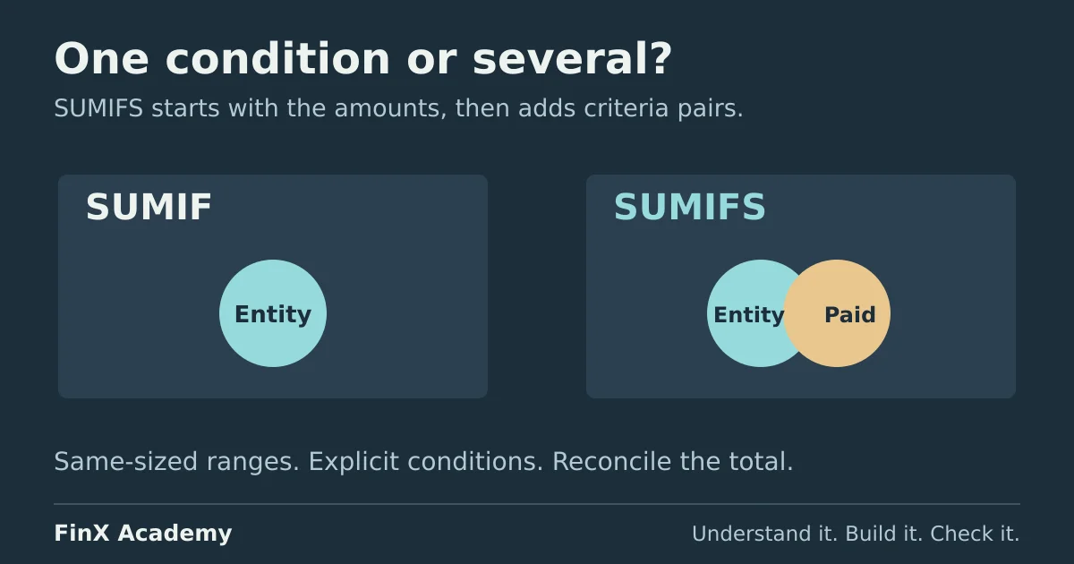
Use SUMIFS as a consistent starting point for conditional totals in new finance work. It accepts up to 127 range/criteria pairs, with all conditions applied together: sum range first, then criteria pairs. SUMIF handles one condition and remains common in inherited files. For one condition and aligned ranges, the two return the same answer — but their argument orders differ, and a swap can produce a plausible zero instead of an error.

Microsoft’s SUMIFS documentation highlights the argument-order difference: SUMIFS requires the sum range first, while SUMIF accepts it as an optional third argument. The invoice ledger below reproduces a mistake, then catches it with a reconciliation.

Compare the two functions before choosing

Decision	SUMIF	SUMIFS
Syntax	SUMIF(range, criteria, [sum_range])	SUMIFS(sum_range, criteria_range1, criteria1, ...)
Conditions	One	One or more, as range/criteria pairs
Sum range	Optional third argument; defaults to the criteria range	Required first argument
Range sizes	Sum range should match the criteria range’s size and shape; otherwise summation starts from its first cell	Every criteria range must have the same number of rows and columns as the sum range

Both come from Microsoft’s SUMIF and SUMIFS references. Because SUMIFS handles a single condition just as well as five, standardising on it keeps one argument order across a workbook and lets a report grow a second condition without rewriting the formula.

Set up the invoice ledger

Use a blank worksheet. These are ten fictional invoices in one currency, entered as positive amounts. Enter the headers in A3:D3 and the records in rows 4–13. Enter column A as real dates, not text:

Row	A: Date	B: Entity	C: Status	D: Amount
4	5 Jan 2026	Northwind	Paid	1,200
5	12 Jan 2026	Blueco	Paid	800
6	20 Jan 2026	Northwind	Open	1,500
7	31 Jan 2026	Blueco	Paid	600
8	3 Feb 2026	Northwind	Paid	900
9	10 Feb 2026	Cedar	Open	2,000
10	14 Feb 2026	Blueco	Paid	750
11	24 Feb 2026	Cedar	Paid	1,100
12	28 Feb 2026	Northwind	Open	400
13	28 Feb 2026	Cedar	Paid	350

Repeated entity names are separate invoices, not duplicates. Keep the source rows visible: every total in this report must be traceable back to them.

Put the report selectors beside the ledger: Entity in F2 with Northwind in G2, and Status in F3 with Paid in G3.

Sum one entity with both functions

First, the single-condition total: every Northwind invoice, whatever its status or date. Reading the source rows, the answer should be 1,200 + 1,500 + 900 + 400 = 4,000. Confirm that by eye before entering any formula.

Put SUMIF: entity in F5 and enter in G5:

=SUMIF($B$4:$B$13,$G$2,$D$4:$D$13)

SUMIF tests the entity names in column B against G2 and adds the aligned amounts from column D. Put SUMIFS: entity in F6 and enter in G6:

=SUMIFS($D$4:$D$13,$B$4:$B$13,$G$2)

Both return 4,000. Notice what moved: the amount range $D$4:$D$13 is SUMIF’s third argument but SUMIFS’ first. The dollar signs keep the ledger fixed if you copy either formula; the absolute-reference guide explains the anchoring pattern.

SUMIF’s optional third argument has one useful effect: with no sum range, it sums the criteria range itself. In an empty cell, =SUMIF($D$4:$D$13,">1000") adds every amount greater than 1,000: 5,800. Microsoft’s SUMIF reference also allows wildcards in criteria — ? matches any single character and * any sequence — which text-matching reports sometimes need.

Add the second condition SUMIF cannot express

Now the report question changes: Northwind invoices that are Paid. The answer is 1,200 + 900 = 2,100. One condition per SUMIF cannot express this; SUMIFS takes a second range/criteria pair. Put SUMIFS: entity + status in F7 and enter in G7:

=SUMIFS($D$4:$D$13,$B$4:$B$13,$G$2,$C$4:$C$13,$G$3)

It returns 2,100. Every range covers the same ten rows — 4 through 13 — which the SUMIFS reference requires: each criteria range must contain the same number of rows and columns as the sum range. Write all three ranges with the same anchors so a copied formula cannot drift onto different rows.

Change G3 to Open and the same formula returns Northwind’s open invoices: 1,500 + 400 = 1,900. Restore Paid before continuing.

Sum a month with explicit date boundaries

Monthly totals need two date conditions: on or after the month’s first day, and before the next month’s first day. Enter the boundary dates as formulas so they cannot be mistyped: Jan start in F8 with =DATE(2026,1,1) in G8, Feb start in F9 with =DATE(2026,2,1) in G9, and Mar start in F10 with =DATE(2026,3,1) in G10. The DATE function builds each serial value from year, month and day.

Put January invoices in F11 and enter in G11:

=SUMIFS($D$4:$D$13,$A$4:$A$13,">="&$G$8,$A$4:$A$13,"<"&$G$9)

Put February invoices in F12 and enter in G12:

=SUMIFS($D$4:$D$13,$A$4:$A$13,">="&$G$9,$A$4:$A$13,"<"&$G$10)

The comparison operator lives inside the quotes and the & joins it to the boundary cell — ">="&$G$8 becomes “on or after 1 Jan 2026”. January returns 4,100 (rows 4–7) and February returns 5,500 (rows 8–13).

Using < next-month-start instead of <= month-end is deliberate. It keeps 31 January inside January without knowing how many days the month has, and it survives timestamps: Excel dates are serial numbers, so a cell holding 31 Jan 2026 16:20 is later than midnight 31 Jan and would fail a <=DATE(2026,1,31) test while still passing < 1 Feb.

Reconcile the filtered totals to the source

A conditional sum is only trustworthy next to a check that does not share its logic. Put Parts total in F14, Source total in F15 and Difference in F16, then enter:

Cell	Formula	Answer
G14	=G11+G12	9,600
G15	=SUM($D$4:$D$13)	9,600
G16	=G14-G15	0

January plus February must equal every invoice, because the two intended windows cover the ledger with no gap and no overlap. A zero difference supports that reconciliation, but does not prove each invoice reached the right month: offsetting omissions and duplicates, or two swapped monthly totals, can still net to zero. Inspect the boundary rows and compare the source dates as well.

Reconcile another cut of the same data: Paid plus Open should also equal the source. With =SUMIFS($D$4:$D$13,$C$4:$C$13,"Paid") returning 5,700 and the same formula with "Open" returning 3,900, the split totals 9,600 as well. Finally, add January’s four rows by hand: 1,200 + 800 + 1,500 + 600 = 4,100. Agreement between formulas is helpful, but the manual addition is what proves the formulas are pointed at the right rows.

Two mistakes that return plausible numbers

Swap the argument order. In an empty cell, write SUMIFS with SUMIF’s order — criteria range first:

=SUMIFS($B$4:$B$13,$D$4:$D$13,$G$2)

This treats the entity names as the values to sum and tests whether each amount equals Northwind. No amount matches a text name, so the result is 0 — no error, no warning. The mirrored SUMIF mistake, =SUMIF($D$4:$D$13,$G$2), omits the sum range and tests amounts against Northwind; it also returns 0. A zero total for a customer you know has invoices is the symptom; the argument order is the cause. Delete both cells afterwards.

Lose a boundary row. Change the January upper bound in G11 from "<"&$G$9 to "<="&DATE(2026,1,30):

=SUMIFS($D$4:$D$13,$A$4:$A$13,">="&$G$8,$A$4:$A$13,"<="&DATE(2026,1,30))

January drops to 3,500 because the 31 Jan Blueco invoice of 600 no longer qualifies. The formula looks correct in isolation; the reconciliation finds it. G14 becomes 9,000 and the difference in G16 becomes −600, which is exactly one invoice. Restore "<"&$G$9 and confirm the difference returns to zero.

This is why the check lives in the report rather than in your head: a date condition that silently excludes one row still returns a number that looks like a month.

Choose the next practice step

Use SUMIFS as the default, anchor every range to the same rows, keep date boundaries as “on or after start, before next start”, and reconcile each filtered total to a sum that does not share its criteria.

The Excel-for-finance budget report applies the same SUMIFS pattern to a departmental report and follows what happens when one condition is removed entirely. If your real task is retrieving one matching record rather than adding many, the XLOOKUP practice covers that difference with missing and duplicate keys, and the INDEX MATCH with multiple criteria guide shows what a first-match retrieval answers — and misses — when a criteria combination repeats.

In FinX’s Excel for Finance course, Mathematical Functions and Anchoring & the Grid are free; the Conditional Aggregation lesson that drills this report pattern requires paid access. Browse the catalogue for current syllabus and pricing, or try the free five-question diagnostic to find the skill to practise next.