A sensitivity grid is useful when each result has a clear pair of inputs. Check its centre, its corners and the direction of change before interpreting it.
Sensitivity analysis shows how a model’s output changes when you vary selected inputs while holding the others constant. In Excel, you can build a small grid with ordinary formulas or use the native Data Table feature to recalculate an existing model.
Start with a result you can calculate independently. This fictional example measures operating profit at different selling prices and sales volumes. The grid shows the consequences of its assumptions; it does not assign probabilities to the outcomes.
Define the model before building the grid
Enter these assumptions in column B, with their labels in column A:
| Cell | Assumption | Value |
|---|---|---|
| B1 | Selling price per unit | 12 |
| B2 | Units sold | 1,000 |
| B3 | Variable cost per unit | 4 |
| B4 | Fixed operating costs | 3,000 |
In B6, calculate operating profit:
=(B1-B3)*B2-B4The base case is (12 − 4) × 1,000 − 3,000 = 5,000. Amounts use one consistent illustrative currency, and the period is one year. Assume all units produced are sold, variable cost per unit stays constant, and fixed costs do not change within the tested volume range. The result excludes interest and tax.
These assumptions matter. A capacity limit, volume discount or change in product mix would require a different model, even if the spreadsheet formulas were entered perfectly.
Build the formula-based sensitivity grid
Put prices of 10, 12 and 14 in D5:F5. Put volumes of 800, 1,000 and 1,200 in C6:C8.
In D6, enter:
=(D$5-$B$3)*$C6-$B$4Copy it across and down to fill D6:F8.
D$5takes the price from row 5; its column changes across the grid.$C6takes the volume from column C; its row changes down the grid.$B$3and$B$4keep the cost assumptions fixed in every result.
The absolute-reference guide explains how to choose which coordinates should move.
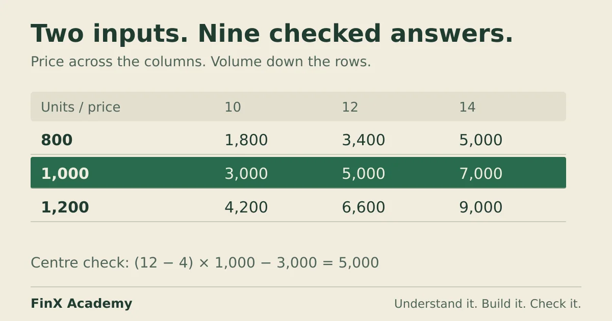
Your completed grid should be:
| Units sold / price | 10 | 12 | 14 |
|---|---|---|---|
| 800 | 1,800 | 3,400 | 5,000 |
| 1,000 | 3,000 | 5,000 | 7,000 |
| 1,200 | 4,200 | 6,600 | 9,000 |
Each cell contains an ordinary formula that can be inspected independently. That makes this approach useful for practising references and reviewing a compact calculation.
Check the centre, corners and direction
The centre cell, E7, must equal the base-case output in B6: both use price 12 and volume 1,000. Then calculate a corner without copying the spreadsheet formula: price 10 and volume 800 give (10 − 4) × 800 − 3,000 = 1,800.
Check how the results move. In this example, a price increase of 2 adds 2,000 to profit at a volume of 1,000. Selling 200 more units adds 1,600 at a price of 12, because the contribution per unit is 8. These checks test the relationships behind the numbers.
Finally, increase fixed costs in B4 from 3,000 to 3,500. Every grid cell should fall by 500. Restore the original assumption afterwards.
Recognise copying mistakes
If you use $C$6 for volume, every row uses 800 units. The top row can look correct while the rows beneath it repeat the wrong answers.
If you use D5 for price, copying down shifts that reference to D6, which contains a calculated profit rather than a selling price. The first row may still work, so checking only D6 misses the error.
Read the copied formula in the bottom-right cell. In F8, the correct formula is:
=(F$5-$B$3)*$C8-$B$4Expected results are checks to compare against. Do not type them over the formulas to make the grid appear correct.
Use Excel’s native two-variable Data Table
A native Data Table substitutes trial values into two input cells of an existing model. To compare it with the formula grid, use a separate area on the same worksheet:
- Enter
=B6inH5, linking to the model’s output. - Put prices 10, 12 and 14 in
I5:K5, and volumes 800, 1,000 and 1,200 inH6:H8. - Select
H5:K8. In desktop Excel for Windows, choose Data → What-If Analysis → Data Table. - Set Row input cell to
$B$1, the original price input. Set Column input cell to$B$2, the original volume input.
The nine results should match the earlier grid. The row and column input fields refer to the model’s assumption cells, rather than the trial-value headers. See Microsoft’s Data Table instructions and Mac instructions for the supported desktop versions and controls.
If results appear stale, check calculation settings and recalculate the table; Microsoft documents an option that excludes Data Tables from automatic recalculation. The ordinary formula grid above does not use that feature.
Interpret the range before adding complexity
The lowest tested profit is 1,800 and the highest is 9,000. Those are the minimum and maximum among these nine combinations, rather than bounds on everything that could happen to the business. Choose ranges that answer a concrete question, and explain why holding the remaining assumptions constant is useful.
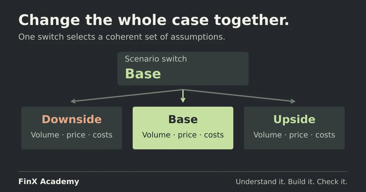
A grid varies one or two inputs with everything else held constant. When the assumptions should move together as a coherent story — base, upside and downside cases — switch the whole model between pre-entered cases instead; the scenario analysis guide builds that switch and the checks that keep the cases from mixing.
FinX’s Sensitivity Without Data Tables lesson teaches formula-based grids. Browse the course catalogue for its scope and access requirements. Native Excel Data Tables are a separate workflow; the lesson does not grade that feature.
Continue with guided practice
Build on this guide with spreadsheet exercises on formulas, lookups and financial functions. Explore the syllabus and start with a free lesson.
Excel for Finance course