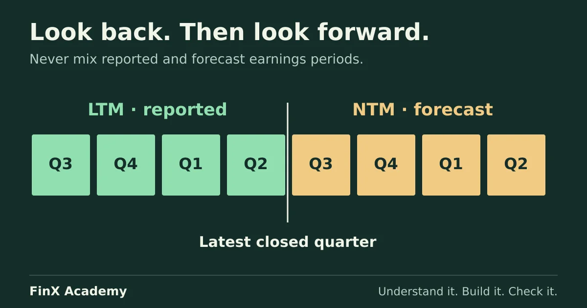
LTM uses the latest reported twelve months; NTM forecasts a stated next-twelve-month window. A multiple comparison is only valid when both sides share the period — mixing bases pays for the growth twice.
LTM (last twelve months, also called TTM) uses the latest reported twelve-month period. NTM (next twelve months) uses a twelve-month forecast. State the start and end dates: a strict forward twelve months from a valuation date can differ from a convention based on the next four financial quarters. LTM is historical reporting, which may contain estimates and adjustments; NTM is a forecast. Both are legitimate denominators — but a peer multiple built on one basis applied to a number built on the other is a silent arithmetic error, not a conservative choice.
This page assembles both periods for Alder, one of the maintenance contractors from the comparable company analysis guide. That page asserts that Alder’s LTM EBITDA is 40.0 and its EV/EBITDA is 7×. Here the 40.0 is built from quarterly data and tied back, then NTM is assembled from a dated fictional forecast and run through the same peer set. Amounts are in millions of one currency.
The rule behind “last twelve months”
The valuation date is 31 August 2026, shared with the comps page. At that date the last closed quarter ends 30 June 2026, so the LTM window is Q3 2025 through Q2 2026 — the exact “LTM through 30 June 2026” convention that page states. We assume those June results are available by 31 August. This article uses a quarter-based forward proxy for NTM: 1 July 2026–30 June 2027. It includes July and August, which have already elapsed by the valuation date but have not been separately reported in this dataset. A strict next twelve months from 31 August would be September 2026–August 2027 and needs monthly or prorated estimates. Keep that difference visible:
- LTM = the last four quarters whose end dates are on or before the valuation date and whose results are reported.
- NTM in these tables = the next four quarters after the latest reported LTM, from a forecast dated 31 August 2026. Use that same convention for every peer and the target.
- If a source instead reports strict date-based NTM, calendarise to a common window before comparing it.
A calendar year, a fiscal year and an LTM are three different twelve-month windows; the “twelve months” in the name guarantees none of them lines up with the others by default.
Enter the quarterly record
The quarter label sits in column B (the cell shown), period-end dates inside it, reported EBITDA in column D and the forecast in column E:
| Row | Quarter, ended | Actual (D) | Forecast (E) | Note |
|---|---|---|---|---|
| 5 | Q1 2025, ended 31 Mar 25 | 8.0 | reported | |
| 6 | Q2 2025, ended 30 Jun 25 | 9.0 | reported | |
| 7 | Q3 2025, ended 30 Sep 25 | 9.0 | reported | |
| 8 | Q4 2025, ended 31 Dec 25 | 11.5 | reported — seasonal peak | |
| 9 | Q1 2026, ended 31 Mar 26 | 9.5 | reported | |
| 10 | Q2 2026, ended 30 Jun 26 | 10.0 | reported — last closed quarter | |
| 11 | Q3 2026, ends 30 Sep 26 | 10.0 | forecast, compiled 31 Aug 2026 | |
| 12 | Q4 2026, ends 31 Dec 26 | 12.0 | forecast | |
| 13 | Q1 2027, ends 31 Mar 27 | 10.5 | forecast | |
| 14 | Q2 2027, ends 30 Jun 27 | 10.5 | forecast |
The company, the quarterly figures and the forecast are fiction; the shape is not — a Q4 peak from winter maintenance work is why this exercise exists at all.
D16  LTM EBITDA  =SUM(D7:D10)   → 40.0
E16  NTM EBITDA  =SUM(E11:E14)  → 43.0
Before reading on: the comps page carries Alder’s LTM EBITDA as 40.0. The sum is 40.0. Sliding one quarter forward and using Q3 2026 forecast gives 11.5 + 9.5 + 10.0 + 10.0 = 41.0, a mixed actual/forecast window. A value of 43.0 instead selects all four forward quarters. Neither is the reported LTM.
Two routes to the same LTM
Quarterly detail is not always available — sometimes you only have the annual report and the latest interim statement. The standard stub-period route then reconstructs the LTM:
LTM = latest full year − same stub last year + this year's stubHere: calendar 2025 total (8.0 + 9.0 + 9.0 + 11.5 = 37.5), minus H1 2025 (8.0 + 9.0 = 17.0), plus H1 2026 (9.5 + 10.0 = 19.5):
=SUM(D5:D8) - SUM(D5:D6) + SUM(D9:D10) → 37.5 − 17.0 + 19.5 = 40.0Two independent routes, one answer: 40.0 — and that answer is the number the comps page asserts, which is why
its 7× (280 ÷ 40) reproduces here exactly. In a real build this is the moment you check your quarter selection
against the published twelve-month figure rather than trusting either alone.
The same company, two multiples
Alder’s enterprise value is 280 (the comps table). Pair it with each denominator:
| Cell | Row | Formula | Result |
|---|---|---|---|
| B17 | Enterprise value | comps table | 280 |
| B18 | EV ÷ LTM EBITDA | =B17/D16 |
7.00× |
| B19 | EV ÷ NTM EBITDA | =B17/E16 |
6.51× |
The NTM multiple is lower — 6.51 against 7.00 — because the company is growing (+7.5% over the window: 43.0 ÷ 40.0). That gap is not a discount; it is the same price divided by a bigger expected base. Holding positive EV constant and using positive earnings, a higher forecast denominator gives a lower multiple, and the two numbers describe one valuation, not two opinions.
Build the NTM range for the peer set
Repeat the NTM forecast for the other peers (fictional, compiled 31 August 2026) and rebuild the comps table on the forward basis. Columns C–F, same four companies:
| Row | Label / formula in C | Alder (C) | Birch (D) | Cedar (E) | Delta (F) |
|---|---|---|---|---|---|
| 22 | EV | 280 | 400 | 540 | 200 |
| 23 | NTM EBITDA | 43 | 53 | 66 | −2 |
| 24 | EV/NTM: =IF(C23<=0,"N/M",C22/C23) |
6.51 | 7.55 | 8.18 | N/M |
Delta’s forecast improves from −5 to −2, and it is still N/M — a forward number can rescue a trend, not a
sign. The median of the three usable multiples, in B26:
=MEDIAN(C24:F24) → 7.55Apply it to the target’s NTM EBITDA of 48.0 (the comps page’s target grown 6.7%): =B26*48 → EV 362.3,
bridge with the comps page’s own terms (minus debt 90, plus excess cash 15, over 20 shares) → equity 287.3,
14.36 per share. The comps page’s LTM route gave 8× × 45 = 360 → 14.25. The consistent per-share answers differ by 0.79%; enterprise values differ by 0.63%.
This reflects the chosen peer and target growth assumptions, not a general tolerance test. Consistent LTM and
NTM valuations can differ substantially when growth, margins or forecasts differ.
Three ways the periods go wrong
1. The mismatched denominator. Take the peer median from the LTM comps table — 8× — and apply it to the target’s NTM EBITDA of 48.0: EV 384, equity 309, 15.45 per share. Against the consistent LTM answer of 360, the overstatement is exactly 6.67% = 48/45 − 1: the target’s own growth rate. The error double-counts it — once because the market already paid for expected growth in the peers’ LTM multiples, and again in your bigger base. This is the failure the comps page warns against in one line (“do not mix LTM earnings for one peer with next-year estimates for another”); here is what the line costs.
2. The roll that forgets to drop. On 12 November 2026 Alder reports Q3 2026 actual EBITDA of 10.2. Update the sheet by adding it under Q3 — and, if the LTM formula was pointed at a five-row range, it now reads 40.0 + 10.2 = 50.2 and the multiple “improves” to 5.58×. A growing LTM that jumps by a full quarter’s EBITDA has become fifteen months. The corrected window drops Q3 2025: 11.5 + 9.5 + 10.0 + 10.2 = 41.2 → 6.80×. Rolling LTM is not “add the new number”; it means sliding the four-quarter frame — and the NTM frame slides with it, now Q4 2026 through Q3 2027.
3. The annualised stub. Only H1 2026 reported and no quarterly detail? Doubling it — 2 × 19.5 = 39.0 — assumes flat quarters, and Alder’s Q4 peak (11.5) sits outside the window. The multiple reads 7.18× instead of 7.00, because the denominator lost exactly the seasonal strength. For a front-loaded business the sign flips and the error flatters the company; annualisation is an estimate, not a reconstruction of reported LTM. Build the window from quarters, or label the stub assumption where the next reader can see it.
Which basis should the headline carry?
Show both when they are useful; otherwise explain the chosen basis. LTM uses reported historical results, but interim figures and adjusted EBITDA are not necessarily audited — but it prices the year that just happened, which for a seasonal or fast-growing business may not resemble any upcoming year. NTM captures ongoing earnings power — but it is somebody’s forecast, so date it, name its source (consensus, management case, your own build) and keep it in its own column. Present both, apply each to its matching denominator, and let the spread carry the information: where LTM and NTM multiples disagree widely, growth or volatility is doing something the other period hides.
Calendarise peers with different fiscal year-ends
Align the period as well as the historical/forecast label. For example, to estimate calendar-2027 EBITDA
from a September year-end company’s FY2027 forecast of 60 and FY2028 forecast of 72, a simple equal-month
weighting gives 9/12*60 + 3/12*72 = 63. That shortcut assumes earnings accrue evenly within each fiscal
year. For seasonal businesses, sum the actual forecast quarters or months that fall in calendar 2027 instead.
Neither calendar-2027 nor this annual weighting automatically equals a strict NTM period from August 2026.
Check your answers
- LTM 40.0 by both routes (quarterly sum; 37.5 − 17.0 + 19.5) — ties to the comps page’s 7× at EV 280.
- NTM 43.0; Alder 7.00× LTM vs 6.51× NTM (+7.5% growth in the denominator).
- Peer NTM multiples 6.51 / 7.55 / 8.18, Delta N/M; median 7.55× → target EV 362.3, 14.36 per share vs the LTM route’s 14.25 (per-share results 0.79% apart; EV results 0.63% apart).
- Errors: mixed basis 384 / 15.45 (+6.67% = the growth rate, twice); five-quarter LTM 50.2 → 5.58× vs correct roll 41.2 → 6.80×; annualised stub 39.0 → 7.18×.
Take the next step
The peer selection, EV construction and target bridge are worked in the comparable company analysis guide; the claim classification behind the bridge sits on the valuation-bridge article; and the DCF model shows a valuation built entirely on explicit forward periods, where the same date-consistency discipline is load-bearing. FinX’s Comps & Precedents course includes a free Choosing the peer set lesson; later lessons require paid access — browse the catalogue for current lessons and access details. The free ten-minute diagnostic asks five numeric modelling questions; it does not grade a calendarised build.
Continue with guided practice
Practise choosing peers, building an enterprise value bridge and interpreting valuation multiples. Explore the Comps & Precedents syllabus and its free lesson.
Comps & Precedents course