DCF model example: build cash flow, terminal value and equity value

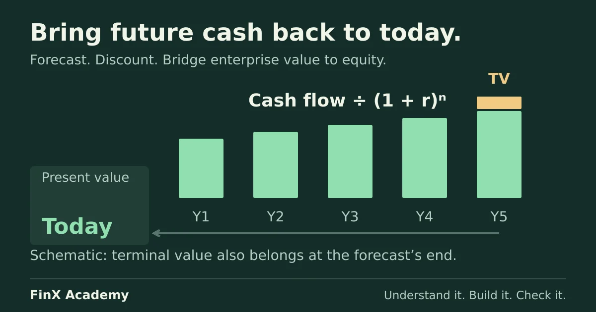
A discounted cash flow (DCF) model estimates value by bringing expected future cash flows back to a valuation date. In this example, five years of operating cash flow plus the value of later cash flows produce an enterprise value of 311.21. Adding excess cash and subtracting debt gives equity value of 266.21.

Those are outputs from fictional assumptions, in millions of one currency. Build the calculation below to see where each number comes from and how an incorrect terminal-value formula overstates the result.

Choose the cash flow and discount rate together

This model uses free cash flow to the firm (FCFF), also called unlevered free cash flow. It measures operating cash available to debt and equity providers after operating taxes and reinvestment, before financing payments:

FCFF = EBIT × (1 − operating tax rate)
       + depreciation and amortisation
       − capital expenditure
       − increase in non-cash operating working capital

EBIT is earnings before interest and tax. Do not deduct interest, debt repayments or dividends from this FCFF calculation. An increase in operating working capital uses cash; cash balances and debt are excluded from that working-capital measure.

For an EBITDA starting point, the unlevered free-cash-flow guide builds a separate worked bridge through tax, D&A and reinvestment.

Discount FCFF at the weighted average cost of capital (WACC), which combines the required returns of debt and equity capital. Cash flow specifically to equity instead needs the cost of equity. Damodaran’s NYU Stern valuation lecture explains why cash flows and discount rates must match.

Enter the five-year forecast

Start at time zero, immediately before Year 1. All forecast cash flows arrive at year-end. Use nominal annual cash flows and rates in the same currency, with these inputs:

Cell	Assumption	Input
B2	WACC, held constant	10%
B3	Perpetual cash-flow growth after Year 5	2%
B4	Simplified operating tax rate	25%

The rates are supplied for this exercise. A company valuation would require evidence for its forecasts, tax treatment and cost of capital; 10% is not a default WACC for every business. The WACC formula guide assembles and audits such a rate from a capital structure, using the same market values as the valuation-bridge article, and the ROIC guide shows how to compare operating returns on book capital with a separately justified cost-of-capital benchmark.

Use columns C:G for Years 1–5. Put labels in column A and enter the period numbers, EBIT, D&A, capex and working-capital increases shown below. Rows 7, 11 and 12 are calculated results:

Row	Label	C: Year 1	D: Year 2	E: Year 3	F: Year 4	G: Year 5
5	Period number	1	2	3	4	5
6	EBIT	40	44	48	52	56
7	After-tax operating profit	30	33	36	39	42
8	D&A	5	5	6	6	7
9	Capex	10	11	12	13	14
10	Increase in operating working capital	5	5	6	6	7
11	FCFF	20	22	24	26	28
12	Present value of FCFF	18.18	18.18	18.03	17.76	17.39

Enter these formulas in column C, then copy across to G:

Cell	Formula	Purpose
C7	=C6*(1-$B$4)	Calculate after-tax operating profit
C11	=C7+C8-C9-C10	Deduct reinvestment after adding back D&A
C12	=C11/(1+$B$2)^C5	Discount that year’s cash flow to time zero

Capex and working-capital increases are entered as positive uses of cash, then subtracted. Keep full precision in formulas and format displayed results to two decimals. The absolute-reference guide explains why $B$2 and $B$4 must stay fixed when you copy across.

Check the explicit forecast value

In B15, enter =SUM(C12:G12). The five forecast cash flows are worth 89.54 today.

Cross-check that result in another empty cell with:

=NPV(B2,C11:G11)

Excel’s NPV function treats the first value as arriving one period after the valuation date and assumes equally spaced, end-of-period cash flows. That matches this exercise. A time-zero payment belongs outside the NPV range; including it would discount it by an extra period. See Microsoft’s NPV documentation.

The equal present values in Years 1 and 2 are intentional: Year 2 FCFF rises by 10%, exactly offsetting one additional year of discounting at 10%.

Calculate terminal value at the right date

Terminal value captures cash flows after Year 5. Assume this fictional business reaches a sustainable cash-flow base at that point, and that the following cash flows can grow at 2% indefinitely after the reinvestment needed to support that growth.

Use the perpetual-growth method:

Cell	Calculation	Formula	Result
B16	Year 6 FCFF	=G11*(1+$B$3)	28.56
B17	Terminal value at end of Year 5	=B16/($B$2-$B$3)	357.00
B18	Present value of terminal value	=B17/(1+$B$2)^G5	221.67
B19	Enterprise value	=B15+B18	311.21

The numerator uses Year 6, the first cash flow beyond the explicit forecast. The terminal value itself sits at the end of Year 5, so discount it for five years. It excludes the Year 5 FCFF already counted in the forecast.

This perpetual-growth formula requires WACC to exceed the growth rate. A positive denominator alone does not justify the assumptions: long-run growth and reinvestment must be sustainable. In a full operating model, forecast those together instead of assuming growth without its cash cost. Damodaran’s terminal-value paper explains these constraints.

The terminal-value comparison applies a trailing exit multiple to this same forecast and checks the growth rate and multiple implied by each method.

Bridge enterprise value to equity value

The 311.21 values the operating business in this example. To find the value attributable to equity, use valuation-date excess cash and debt:

Cell	Item	Input or formula	Result
B21	Excess cash, outside operating needs	15	15.00
B22	Debt value	60	60.00
B23	Equity value	=B19+B21-B22	266.21

Assume there are no other non-operating assets or claims. A real bridge may also need adjustments for investments, non-controlling interests, preferred capital or other claims. The NYU Stern lecture’s equity bridge illustrates these adjustments.

Do not subtract Year 5 debt from today’s enterprise value, or add forecast cash that the DCF already captures. Use the debt-schedule guide to understand principal movements before connecting debt balances.

Diagnose the terminal-value mistake

Replace B19 temporarily with =B15+B17. Enterprise value jumps to 446.54. The model has added a Year 5 value directly to today’s forecast value, overstating enterprise value by 135.33.

Restore =B15+B18. A useful check is that a positive future terminal value has a lower present value when the discount rate is positive: here, 221.67 < 357.00.

Next, increase only Year 1 capex from 10 to 11. Year 1 FCFF should fall from 20 to 19, and enterprise value should fall by 1/1.10, or 0.91. Later forecast flows and terminal value stay unchanged because their inputs are fixed in this exercise. Restore capex to 10 before the next step.

Test WACC and perpetual growth

About 71% of the base enterprise value comes from the present value of terminal cash flows. Small changes in long-run assumptions therefore deserve attention.

Change B2 and B3 to each pair below and record B19. Keep the five explicit forecast cash flows unchanged; the terminal numerator updates with growth. Each table entry is enterprise value, not equity value:

WACC / perpetual growth	1%	2%	3%
9%	321.77	357.19	404.42
10%	284.65	311.21	345.36
11%	254.99	275.49	301.11

At fixed growth, a higher WACC lowers value. At fixed WACC, higher perpetual growth raises value under this cash-flow assumption. The base case is the centre cell. Subtract 45 from any entry to apply this example’s unchanged cash-and-debt bridge.

This grid shows mechanical sensitivity, not probabilities or a confidence interval. A full scenario would also revisit the operating forecast and reinvestment required by different growth assumptions. The Excel sensitivity guide explains how to build and check a reusable grid.

For the forecast connections behind FCFF, continue with the three-statement model example. FinX’s Financial Modeling & Valuation course includes DCF practice with paid access; browse the catalogue for the current lessons.

The football-field guide shows how to compare a DCF range with trading comps and precedent transactions while keeping dates and claim definitions consistent.