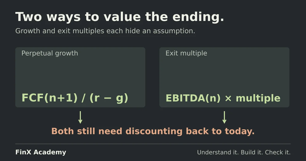
Both terminal-value formulas answer the same question — what is the business worth at the end of the forecast — so report the other method's implied assumption with every number: the multiple behind your growth rate, the growth rate behind your multiple.
Terminal value is what the cash flows beyond your explicit forecast are worth, stated at the end of the forecast period. Two formulas dominate practice: the perpetual growth (Gordon growth) formula and the exit multiple. They are not two opinions about price; they are two assumptions about the future, and each one hides the other’s assumption inside it. This article runs both on one fictional forecast, converts each answer into the other’s terms, and shows where the growth formula breaks.
The example continues the company from the DCF model guide: Year 1–5 free cash flow to the firm of 20, 22, 24, 26 and 28 (millions), Year-5 EBITDA of 63, a 10% WACC and a five-year horizon with year-end cash flows. That guide owns the full build and the equity bridge; this page starts where it ends.
Put the shared inputs on one sheet
| Cell | Label | Value |
|---|---|---|
B2 |
WACC | 10% |
B3 |
Perpetual growth rate | 2% |
B4 |
Exit multiple (EV/EBITDA) | 7.0 |
C6:G6 |
FCFF, Years 1–5 | 20 · 22 · 24 · 26 · 28 |
G7 |
Year-5 EBITDA | 63 |
In B8, value the explicit period: =NPV(B2,C6:G6) returns 89.54 — Excel’s NPV discounts the first flow one full period, which matches year-end timing. The rates and flows are supplied for the exercise; a real valuation has to evidence them.
Method 1: perpetual growth
The formula values a growing stream that never ends:
TV(end of Year 5) = FCFF₅ × (1 + g) ÷ (WACC − g)In Excel:
| Cell | Formula | Result |
|---|---|---|
B10 |
=G6*(1+B3) |
28.56 |
B11 |
=B10/(B2-B3) |
357.00 |
B12 |
=B11/(1+B2)^5 |
221.67 |
B13 |
=B8+B12 |
311.21 |
B14 |
=B12/B13 |
71.2% |
Three rules hide in those cells, and the DCF build proves each one mechanically: the numerator is Year 6’s cash flow — the first flow beyond the forecast, never the Year-5 figure already counted; the result sits at the end of Year 5, so it is discounted five years like any other future amount; and the whole formula requires g < WACC — the denominator is what the next sections test. The present value of terminal cash flows is 71.2% of enterprise value here. That makes the terminal assumptions central to this result; the size of the share does not validate them.
Method 2: exit multiple
The alternative estimates the operating business’s value at the horizon using a valuation multiple. It does not require an actual sale:
TV(end of Year 5) = Year-5 EBITDA × exit multipleIn B16 enter =G7*B4: 441.00. Then discount and combine exactly as before — =B16/(1+B2)^5 gives 273.83 (B17), enterprise value =B8+B17 is 363.37 (B18), and the terminal share is 75.4% (B19).
Two conventions matter. This example uses a trailing EV/EBITDA multiple at the end of Year 5, so it applies to Year-5 EBITDA. A forward multiple would instead use the corresponding forecast period, such as Year 6; match the period to the multiple’s definition. And the terminal value is future money: a common slip is to treat exit proceeds as “just a number from a market” and forget the five-year discount; changing B17 to =B16/(1+B2)^4 returns 301.21 and overstates value by 27.38. The multiple itself is an assumption, not a fact borrowed from today’s market — Damodaran’s terminal-value paper notes that a multiple-based terminal value imports relative valuation into a DCF. Where a defensible range comes from is the comparable-company analysis.
The two answers differ — find the assumption that explains it
Same company, same forecast, same discount rate, and the methods disagree: 363.37 against 311.21, a 52.16 (16.8%) difference in enterprise value. Terminal value is method-sensitive, and the reconciliation is two more cells.
What growth rate is the 7.0× really assuming? Rearranging the perpetuity formula — solving 441.00 = 28×(1+g)/(0.10−g) for g — gives:
implied g = (TV × WACC − FCFF₅) ÷ (TV + FCFF₅)
          = (441.00 × 0.10 − 28) ÷ (441.00 + 28) = 16.10 ÷ 469 = 3.43%
Substitute the unrounded rate — approximately 3.4328% — back into Method 1 and the terminal value is 441.00 again, exactly. A 7.0× exit that sounds like “a normal market multiple” is, under these cash flows, equivalent to free cash flow growing at 3.43% every year forever under the simplified perpetuity assumptions: 1.4 points faster than the 2% the perpetuity case assumed, and a rate you would have to defend as sustainable in perpetuity rather than for the next few years.
What multiple does the 2% really assume? In B21, =B11/G7 divides the perpetuity’s 357.00 by Year-5 EBITDA: 5.67×. Under this forecast and WACC, the 2% perpetuity value is equivalent to 5.67× Year-5 EBITDA. The equivalence changes if the sustainable cash-flow base or reinvestment assumptions change.
That pair — implied multiple and implied growth — is the check a reviewer runs first. Neither method is “the right one”: use both, let comparable evidence bound the multiple (comparable-company analysis), and quote whichever implied assumption you are unwilling to defend. Also keep the metrics straight: the perpetuity uses FCFF, already net of the reinvestment growth costs, while the multiple uses EBITDA, before tax and capex — one reason the conversions never line up “by themselves”.
When the growth formula breaks
Set the perpetual-growth cell B3 to each of these and watch B11:
B3 |
=B10/(B2-B3) returns |
What it means |
|---|---|---|
| 10% | #DIV/0! |
WACC − g = 0: a stream growing as fast as the discount rate has no finite value. |
| 11% | −3,108.00 | Negative denominator: enterprise value becomes −1,840.28. A negative terminal value is impossible for a business that still generates positive cash — the formula is answering a question you didn’t ask. |
| 9% | 3,052.00 | No error at all — and that is the dangerous one. The denominator is a thin 1%, so value is 1,984.59 with 95.5% of it terminal. Every conclusion now rests on one decimal place. |
g < WACC is necessary for this positive growing perpetuity to have a finite value, but it does not establish economic plausibility. Damodaran’s terminal-value guidance constrains stable growth by the economy’s long-run growth, matching the currency and real or nominal basis; his rule of thumb is not to exceed the risk-free rate used in the valuation. The 2% here is an illustrative input, not a verified GDP forecast or an automatically defensible choice.
The terminal cash flow also needs enough reinvestment to support the assumed growth, and terminal risk should reflect a mature business. Our implied 3.43% holds the Year-5 cash-flow base fixed. If sustaining that growth requires more capex or working capital, rebuild terminal FCFF before relying on the conversion.
Make the terminal value state its assumptions
Before a DCF leaves your hands: terminal value sits at the end of the last forecast year and gets the full five-year discount whichever method produced it; the perpetuity numerator is Year 6; =NPV(...)-style checks tie the explicit period; the terminal share (71.2% / 75.4% here) is quoted out loud; and both implied assumptions — 5.67× and 3.43% above — have been calculated. Restore B3 to 2% after the failure cases. Then test the spread mechanically: an exit multiple from 6.0× to 8.0× moves enterprise value from 324.25 to 402.48, so the sensitivity grid belongs next to the assumption cells, and the DCF model guide shows the full build around them.
To find where your own assumptions break first, take the free five-question modeling test — five questions in ten minutes, marking numeric answers, not a graded workbook — or browse the course catalogue for the DCF practice and current access requirements.
Continue with guided practice
Put the valuation concepts into practice with exercises on financial statements, forecasts and DCF valuation. View the syllabus and try a free lesson.
Financial Modeling & Valuation course