Comparable company analysis: build a peer set and valuation range

Comparable company analysis, or trading comps, estimates a business’s value from the market valuations of comparable listed companies. You select peers, calculate consistent valuation multiples, and apply a defensible range to the business being valued.

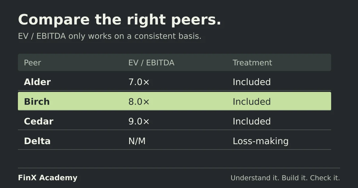
In this fictional example, three usable EV/EBITDA multiples are 7×, 8× and 9×. Applying them to the target business gives enterprise values of 315–405 and equity values of 240–330, in millions. A fourth peer has negative EBITDA: keeping its limitation visible is part of the analysis.

Write the peer-selection rule first

Our target is a regional industrial-maintenance business serving commercial customers through recurring service contracts. For this exercise, screen for a similar customer base, geography, labour and equipment requirements, and scale. Then compare growth, margins and operating risk before selecting a multiple.

Use this fictional candidate review:

Candidate	Operating comparison	Treatment
Alder, Birch and Cedar	Regional maintenance providers with similar scale, contract mix, growth and positive margins to the target	Retain for the worked EV/EBITDA comparison
Delta	Meets the operating screen but currently has losses	Keep visible; its negative EBITDA cannot support this positive-earnings multiple comparison
Orbit Software	Sells maintenance software; materially different delivery costs, growth and cash-generation pattern	Exclude from this operating peer set before calculating its multiple

The assumptions make the teaching example small enough to reproduce. In real research, support the screen with filings, segment data and operating metrics; do not merely describe companies as similar. Record exclusions before seeing which selection produces the preferred value.

Damodaran’s NYU Stern discussion of comparable firms focuses on similar growth, risk and cash-flow characteristics. Sharing an industry label is only a starting point.

Align the dates, units and earnings definition

EBITDA means earnings before interest, taxes, depreciation and amortisation. Use these conventions for every peer and the target:

• Share prices use one illustrative valuation date: 31 August 2026.
• EBITDA covers the same last twelve months (LTM) through 30 June 2026. Assume those reports were available by the valuation date and the supplied debt/cash figures reflect known changes by then.
• Money and share counts are in millions, except share prices. A price of 12 multiplied by 20 million shares gives equity value of 240 million.
• Cash means excess cash outside operating needs. Assume no options, preferred shares, non-controlling interests, lease liabilities or other bridge adjustments.
• EBITDA has the same definition across the set. The figures are already on a consistent basis for this exercise.

For real companies, reconcile adjustments and accounting differences rather than assuming every “adjusted EBITDA” label means the same thing. Do not mix LTM earnings for one peer with next-year estimates for another. EBITDA also omits cash costs such as capex and working-capital investment; similar EBITDA does not establish similar free cash flow.

Build enterprise value before the multiple

Enterprise value (EV) and EBITDA both relate to the operating business before financing costs. Pairing equity value with EBITDA mixes different claims on the business. The NYU Stern consistency tests for multiples explain this matching principle.

Put the four peer names in C3:F3, row labels in column A, and enter the inputs below. Rows 6, 9 and 11 are calculated results:

Row	Label	C: Alder	D: Birch	E: Cedar	F: Delta
4	Share price	12	18	20	10
5	Shares outstanding	20	20	25	15
6	Equity value	240	360	500	150
7	Debt	70	80	110	60
8	Excess cash	30	40	70	10
9	Enterprise value	280	400	540	200
10	LTM EBITDA	40	50	60	−5
11	EV/EBITDA	7×	8×	9×	N/M

Enter these formulas in column C and copy across through column F:

Cell	Formula	Purpose
C6	=C4*C5	Market equity value
C9	=C6+C7-C8	Add debt and subtract excess cash
C11	=IF(C10<=0,"N/M",C9/C10)	Calculate a usable multiple for positive EBITDA

Keep the multiples numeric: the result in C11 is 7, with “×” used only as a display label. Do not type 7x into a calculation cell as text.

For Alder, (240 + 70 − 30) ÷ 40 = 7×. Using only equity value would give 240 ÷ 40 = 6×; that is not its EV/EBITDA multiple.

The formula assumes complete numeric inputs. Flag missing financial data separately instead of treating it as a genuine zero or using a blanket error-to-zero formula.

Keep N/M out of the arithmetic, but in the explanation

Delta’s EBITDA is −5. Dividing EV of 200 by it produces −40× mathematically, but that number does not describe a cheap positive-earnings business. Display N/M, meaning “not meaningful,” for this comparison. The same formula flags zero EBITDA, for which division is undefined.

In B14, calculate:

=MEDIAN(C11:F11)

The answer is 8×, the middle of 7, 8 and 9. Excel ignores text in a referenced range, including the formula-produced N/M text, while including numeric zero. See Microsoft’s MEDIAN documentation.

State the sample clearly: three numeric multiples from four operating peers. The statistic represents the profitable subset. Investigate Delta’s losses and whether they signal risks relevant to the target; excluding an unusable ratio does not make those risks disappear.

Apply the range and bridge to equity

Enter these target inputs:

Cell	Input	Value
C17	Target LTM EBITDA	45
C18	Target debt	90
C19	Target excess cash	15
C20	Target shares	20

For this mechanical example, use the lowest, median and highest usable peer multiples. Enter 7 in C23, =$B$14 in D23, and 9 in E23. Build the output:

Row	Calculation	C: 7×	D: 8×	E: 9×
24	Enterprise value	315	360	405
25	Equity value	240	285	330
26	Implied value per share	12.00	14.25	16.50

Use these formulas, then copy across to E:

Cell	Formula
C24	=C23*$C$17
C25	=C24-$C$18+$C$19
C26	=C25/$C$20

At the median, 8 × 45 = 360 enterprise value. Subtract debt of 90 and add excess cash of 15 to get 285 equity value. Divide by 20 million shares to get 14.25 per share. The DCF model example uses the same bridge after estimating operating value through discounted cash flows.

The 7–9× span describes this selected sample. It is not a confidence interval or an automatic fair-value range. The target’s growth, margins, investment needs and risks determine whether a premium or discount is supportable. A low multiple alone does not establish that a company is undervalued.

Break the median and trace the effect

Temporarily replace Delta’s N/M in F11 with numeric 0. The four numbers become 0, 7, 8 and 9, so the median falls to 7.5×: (7 + 8) ÷ 2.

Because D23 links to the median, the middle-case enterprise value falls to 337.5, equity value to 262.5, and per-share value to 13.13 when displayed to two decimals. The equity result is now 22.5 lower solely because an unusable ratio became a false numeric observation. Restore the formula in F11; the median should return to 8×.

Now test the target bridge independently. Increase debt in C18 from 90 to 100, holding EBITDA and the selected multiples fixed. Middle-case enterprise value stays 360, equity value falls to 275, and per-share value becomes 13.75. If enterprise value changes too, inspect the formula references. Restore debt to 90 afterwards.

Use comps alongside the operating model

Trading comps reflect how the selected public peers are priced at a particular date. They do not establish what an acquirer would pay, and market pricing across the whole peer group can be optimistic or pessimistic. Compare the result with the assumptions in a DCF valuation, and use the sensitivity-analysis guide to explore changes in EBITDA and the selected multiple.

FinX’s Comps & Precedents course includes a free Choosing the peer set lesson; later lessons require paid access. Browse the catalogue for current lessons and access details.

Continue with precedent transactions to compare acquisition prices for this target, LTM vs NTM to build and align the earnings periods, and unlevered beta to separate business risk from leverage in the fictional peer data. The football-field guide explains how to chart ranges on one basis.