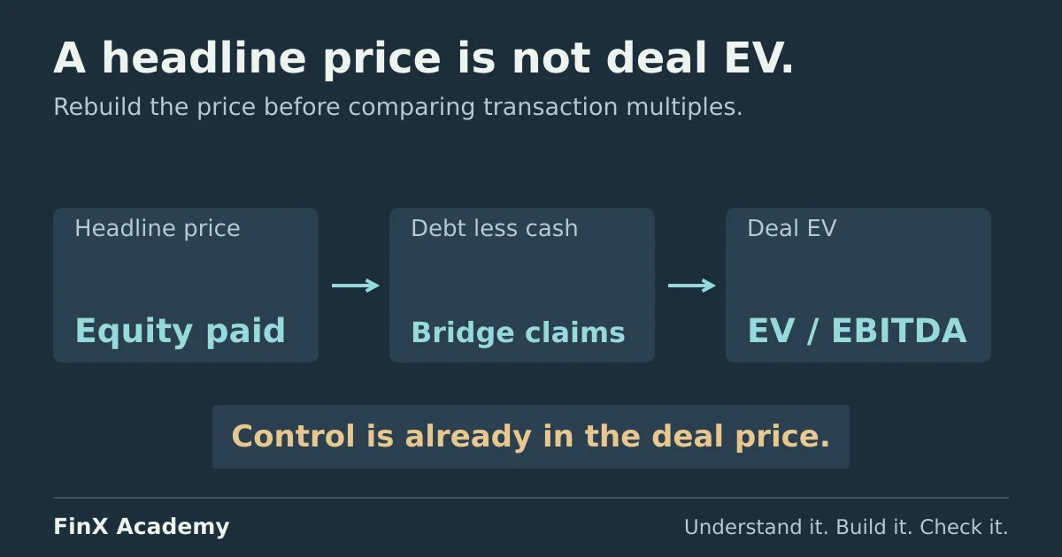
A deal multiple prices control, so never stack a premium on top. Rebuild every headline price into enterprise value on one consistent basis, keep missing data visible as N/M, and state which deals the statistic actually uses.
Precedent transaction analysis values a business from consideration agreed in comparable acquisitions for similar businesses. It is the deal-data twin of comparable company analysis: same style of multiple, same bridge, different evidence — a negotiated purchase of the whole business, not a trading price of a minority stake.
This page runs the analysis for the same regional industrial-maintenance business as the comps article — LTM EBITDA 45.0, debt 90.0, excess cash 15.0, 20.0 million shares — over five explicitly fictional deals announced between August 2024 and November 2025. Amounts are in millions of one currency. The valuation date is 31 August 2026; all five deals are assumed completed by that date. We use announced consideration, held unchanged at completion in this example. Every figure is invented; every cell is auditable.
Write the deal-selection rule first
Screen deals the way the comps article screens peers: similar customer base, delivery model, scale and contract mix. Then check the deal itself before trusting its multiple.
| Deal | Comparison | Treatment |
|---|---|---|
| Aldergate, Colebrook and Enderby facilities groups | Regional maintenance providers of similar scale and contract mix, sold as going concerns | Retain for the worked EV/EBITDA comparison |
| Garland Technical Services | Meets the operating screen; the private seller never disclosed earnings | Keep visible; a blank EBITDA gives N/M, not a guess |
| PipeWire scheduling software | Sold for recurring subscription economics, materially different costs and growth | Exclude before calculating, the same basis as Orbit Software in the comps peer set |
Record the exclusions before seeing which selection produces the preferred value. A deal set small enough to hand around is small enough for one inclusion to move the answer — that fragility gets its own section below.
Rebuild each headline price into enterprise value
A headline may quote equity consideration or enterprise value. Read its definition before building a bridge.
Here the supplied headlines are explicitly 100% equity consideration. The multiple’s numerator is enterprise value: what it takes to own
the whole business, the same distinction the
valuation-bridge article drills for a live company. Put deal names in
C3:F3 and row labels in column A:
| Row | Label | C: Aldergate | D: Colebrook | E: Enderby | F: Garland |
|---|---|---|---|---|---|
| 4 | Announced | 14 Feb 2025 | 20 Aug 2024 | 3 Nov 2025 | 26 Jun 2025 |
| 5 | Offer to shareholders (equity) | 300 | 240 | 380 | 300 |
| 6 | Plus target debt | 55 | 45 | 60 | 50 |
| 7 | Less target cash | 15 | 15 | 20 | 20 |
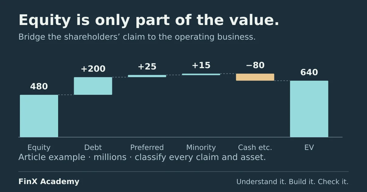
| 8 | Enterprise value | 340 | 270 | 420 | 330 |
| 9 | LTM EBITDA — numeric input | 40 | 30 | 40 | (blank) |
| 11 | LTM period end — date label | 30 Sep 2024 | 30 Jun 2024 | 30 Jun 2025 | undisclosed |
| 10 | EV/EBITDA | 8.5× | 9.0× | 10.5× | N/M |
Enter these formulas in column C and copy across to column F:
| Cell | Formula | Purpose |
|---|---|---|
| C8 | =C5+C6-C7 |
Bridge the equity offer to enterprise value |
| C10 | =IF(ISNUMBER(C9),IF(C9>0,C8/C9,"N/M"),"N/M") |
Calculate a usable multiple only for numeric positive EBITDA |
The outer ISNUMBER check excludes blanks and text; the inner check excludes zero and negative EBITDA.
Keep dates in row 11 rather than typing 40 (Sep 2024) into a numeric cell. Before calculating, verify that
rows 5–7 are numeric too. There are no preferred claims, minority interests, contingent payments or lease
adjustments in this simplified dataset; a real deal may require those additional bridge rows.
One date convention, stated once and applied to every deal: EBITDA is the LTM figure ending at the target’s most recently reported period before the announcement. Row 11 therefore records each figure’s period end, so the reader can see what “LTM” meant on each deal’s date — an unlabeled set of trailing figures is the deal-table version of the mismatched-period error. For real research, source these rows from filings and deal databases, and record what the acquirer disclosed about assumed debt and cash at completion.
DecisionPoint’s SEC-filed transaction analysis illustrates disclosed selection criteria and the use of public transaction and LTM financial information. It is evidence of the research process, not a source for this fictional deal set.
Take the statistics from the usable set
Label the median in A13 and compute it in B13:
- Median:
=MEDIAN(C10:F10)→ 9.0×, the middle of 8.5, 9.0 and 10.5. - Range:
=MIN(C10:F10)and=MAX(C10:F10)→ 8.5× to 10.5×; both ignore the N/M text, like MEDIAN. See Microsoft’s MEDIAN documentation.
State the sample with the statistic: three usable multiples from four recorded deals, five reviewed. The numbers describe the deals that survived the screens, nothing more.
Before reading on: three points 8.5, 9.0 and 10.5 — the median of an odd count must be one of the observed points
and must sit between the extremes. Anything in B13 that is not exactly one of the three is a wiring error,
whatever the formula says.
Apply the range and bridge to equity
The target inputs match the comps article cell for cell: LTM EBITDA 45.0 in C17, debt 90.0 in C18, excess cash
15.0 in C19, shares 20.0 in C20. Enter 8.5 in C23, =$B$13 in D23 (link the median — never retype it) and
10.5 in E23, then:
| Row | Calculation | C: 8.5× | D: 9.0× | E: 10.5× |
|---|---|---|---|---|
| 24 | Enterprise value | 382.5 | 405.0 | 472.5 |
| 25 | Equity value | 307.5 | 330.0 | 397.5 |
| 26 | Implied value per share | 15.38 | 16.50 | 19.88 |
The formulas are the comps article’s, unchanged: =C23*$C$17, =C24-$C$18+$C$19, =C25/$C$20. At the median,
9.0 × 45.0 = 405.0 enterprise value, less debt 90.0 plus cash 15.0 is 330.0 equity, or 16.50 per share.
(The low and high per-share results are exactly 15.375 and 19.875, displayed to two decimals.)
Set the two ranges side by side for the same business:
| Method | Multiples | Enterprise value | Equity value | Per share |
|---|---|---|---|---|
| Trading comps (three usable peers) | 7×–9×, median 8× | 315–405 | 240–330 | 12.00–16.50 |
| Precedent deals (three usable deals) | 8.5×–10.5×, median 9.0× | 382.5–472.5 | 307.5–397.5 | 15.38–19.88 |
Why deal and trading prices can differ
An acquirer’s price buys control: the right to appoint the board, set the dividend and sell the assets. Public share prices usually reflect trades in minority stakes. Deal prices also embed expected synergies, competitive tension between bidders, and the scarcity of assets actually for sale. Those factors can lift deal multiples, although distress, deal terms and market conditions can also lower them. The comps article warns that trading multiples “do not establish what an acquirer would pay” — here the precedent median of 9.0× sits 12.5% above the trading median of 8.0×, and the precedent range of 8.5–10.5× overlaps only the top quarter of the trading range of 7–9×.
Two cautions, in both directions:
- Never stack a premium on top of a precedent multiple. The control premium is already inside 8.5–10.5; paying it again double-counts. A control adjustment to trading comps also needs transaction-specific support; it is not an automatic uplift.
- 12.5% is not a takeover premium measurement. It compares the medians of two different distributions — peer trading multiples here, deal multiples there — over different populations and dates. Measured premia come from the target’s own pre-announcement share price against its offer, and published studies of those show wide spreads by market and era. This exercise has no observable share price for the target; do not invent one.
Break the analysis and trace the effect
1. The headline price goes straight into the numerator. Replace Colebrook’s EV of 270 with the equity offer of
240 and its multiple becomes 240 ÷ 30 = 8.0×. The usable set is now 8.0, 8.5 and 10.5, so the median falls to
8.5× — and 8.5 is still inside the old range, which is what makes the error travel so quietly. Median enterprise
value drops to 382.5, equity to 307.5, per share to 15.38: the answer falls by 22.5 of equity value, 1.125 per
share, from one missing bridge. Note the signature: the tampered multiple lands at a plausible-looking 8.0×, close
to the trading median. Plausibility is not agreement — keep the bridge as its own row and retrace it: 240 is the full equity purchase price, including whatever control value was negotiated; it omits net
debt. EBITDA is a pre-financing measure, so it pairs with enterprise value, not that equity price.
2. A guessed number completes the set. Garland’s EBITDA is blank and its multiple reads N/M. Suppose you “use a
rule of thumb” and type 27.5 (so the deal prints 12.0×). The four points are 8.5, 9.0, 10.5 and 12.0; the median
becomes (9.0 + 10.5) ÷ 2 = 9.75×, median enterprise value rises to 438.75 and equity to 363.75 — the
whole valuation shifts by 33.75 on one invented figure. The N/M keeps that deal out of the arithmetic while keeping
it visible in the explanation, exactly as Delta’s negative EBITDA does in the comps article. Investigate Garland’s
earnings instead; if they stay undisclosed, say so in the memo.
3. A different period slips into one row. Enderby’s 10.5× divides 420 by the LTM EBITDA of 40.0 for the period ending 30 June 2025. Suppose you instead divide by 45.0 — the forward figure an analyst expected after the deal closed — and record 9.3×. The set becomes 8.5, 9.0 and 9.3, and the median stays 9.0× to the letter: one corrupted row moves the maximum but not the headline. That is the trap the median sets in a three-point sample — it hides single-row basis drift, so the check has to be per deal: same numerator definition, same trailing-earnings definition, same date convention, on every row, before any summary statistic is trusted.
Check your answers
- Enterprise values 340, 270, 420, 330; multiples 8.5×, 9.0×, 10.5×, N/M.
- Median 9.0×; range 8.5–10.5×; three usable multiples from four recorded deals, five reviewed.
- Implied values at 8.5× / 9.0× / 10.5×: EV 382.5 / 405.0 / 472.5, equity 307.5 / 330.0 / 397.5, per share 15.38 / 16.50 / 19.88.
- Trading-comps comparison: medians 8.0× vs 9.0×, a 12.5% gap — not a measured control premium.
- Breaks: equity-as-EV → median 8.5×, equity 307.5 (−22.5); guessed 27.5 → median 9.75×, equity 363.75 (+33.75); forward-EBITDA Enderby → row reads 9.3×, median unchanged at 9.0× — the summary statistic misses it.
Take the next step
The comparable company analysis guide prices the same target off peer trading multiples — keep the two ranges side by side and defend the gap. The enterprise value vs equity value bridge owns the claim-by-claim reasoning behind every row-8 formula above, and the football-field guide puts ranges on a consistent chart. The DCF model values a business from its own cash flows rather than anyone else’s price. FinX’s Comps & Precedents course includes a free Choosing the peer set lesson; later lessons require paid access — browse the catalogue for current lessons. The free ten-minute diagnostic asks five numeric modelling questions; it does not grade a deal table.
Carry the agreed price into the sources and uses table to calculate acquisition funding and audit the equity contribution.
Continue with guided practice
Practise choosing peers, building an enterprise value bridge and interpreting valuation multiples. Explore the Comps & Precedents syllabus and its free lesson.
Comps & Precedents course