Football field valuation: build and check a valuation chart

A football field valuation is a chart of valuation ranges from several methods on a common scale. Trading comparables, precedent transactions and a discounted cash flow model can each supply a bar. The chart helps a reader compare their conclusions without hiding which assumptions produced each range.

Build the underlying analyses first. The DCF guide, comps guide and precedent-transactions guide explain those methods. This page handles the chart: input ranges, floating-bar geometry, one enterprise-to-equity bridge, and checks on the interpretation.

Set one date and one claim basis

The example uses fictional Northgate Logistics at 31 August 2026. All amounts are in millions of one currency. The valuation bridge supplies market equity of 480.0, gross debt 200.0, excess cash 80.0, preferred shares 25.0, minority interest 15.0 and 20.0 million common shares:

Bridge deductions = 200 − 80 + 25 + 15 = 160
Market enterprise value = 480 + 160 = 640
Market share price = 480 / 20 = 24.00

Every bar below is enterprise value, with the same claims included. A chart can instead use equity value or value per share, but all bars must be converted to that same basis. Align valuation dates, currencies and earnings periods before comparing methods.

Enter the assumptions and their sources

Cell	Input	Value
B2	LTM EBITDA	80.0
B3	Low trading multiple	7.0×
B4	High trading multiple	9.0×
B5	Low precedent multiple	8.5×
B6	High precedent multiple	10.5×
B7	Bridge deductions	160.0
B8	Year-1 FCFF	42.0
B9	Assumed aggregate WACC	8.5%
B10	Perpetual FCFF growth	2.0%
B11	WACC sensitivity, plus/minus	0.5%
B12	Market EV reference	640.0

Enter multiples as numbers such as 7, not text such as 7x. B11 stores 0.005: a 0.5-percentage-point change, not a 0.5% relative change in WACC.

The 80.0 EBITDA and 160.0 bridge come from Northgate’s valuation example. The 42.0 is the next-year cash flow assembled in the FCFF guide. The multiple endpoints reuse the fictional maintenance-sector examples in the comps and precedent guides only to demonstrate the chart. They are not established comparable ranges for a logistics business; a real Northgate valuation needs a suitable peer and deal screen.

The 8.5% WACC is a new illustrative aggregate discount-rate assumption for the claims represented by this EV. It is not derived from the two-component WACC example, which excludes preferred and minority claims. A real analysis must support the discount rate and claim coverage consistently. The CAPM guide shows one source of uncertainty in that rate.

To keep the chart example small, the DCF bar uses a growing perpetuity starting with Year-1 FCFF. We assume that 42.0 can grow 2% annually after the reinvestment required to support that growth. This is a simplified scenario, not the five-year forecast from the DCF article. With FCFF1 already in B8, its present value is:

EV = FCFF1 / (WACC − g)

Do not multiply B8 by (1+g) again. That would use Year-2 cash flow one year too early. A formula starting from current-year FCFF0 would need that growth step; the terminal-value guide explains the timing distinction.

Calculate each range

Create the following table in A16:E19. C and D hold low and high EV; E is the width, =D17-C17, copied down.

Row	Method (A)	Low EV (C)	High EV (D)	Width (E)
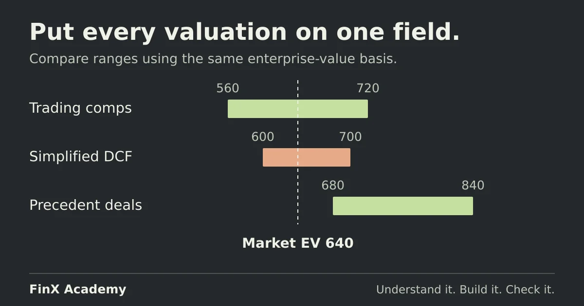
17	Trading comps	=$B$2*$B$3 → 560.0	=$B$2*$B$4 → 720.0	160.0
18	Simplified DCF	=$B$8/($B$9+$B$11-$B$10) → 600.0	=$B$8/($B$9-$B$11-$B$10) → 700.0	100.0
19	Precedent deals	=$B$2*$B$5 → 680.0	=$B$2*$B$6 → 840.0	160.0

The DCF low is 42/(9%−2%) = 600; the high is 42/(8%−2%) = 700. Higher WACC gives lower value. The central-rate result is 42/(8.5%−2%) = 646.15, which is not the endpoints’ midpoint of 650.00. A nonlinear valuation does not generally put the base case at the centre of its sensitivity range.

Draw the football field in Excel

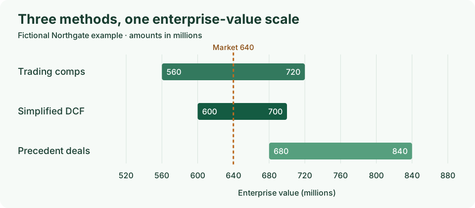
Use a stacked horizontal bar chart with two series: Low and Width. The Low series is the invisible base; Width is the visible range. This follows the floating-bar technique in Microsoft’s stacked-bar walkthrough.

1. Select the three method labels, Low values and Width values. Insert a stacked bar chart, with Low first and Width second. Do not plot High as the second series.
2. Set Low to no fill and no border. The visible Width then begins at Low and ends at Low + Width = High.
3. Set the horizontal value axis to minimum 520, maximum 880 and a major unit of 40. Leave Low as its absolute value — do not subtract the axis minimum. Axis bounds change the visible window, not the data.
4. Reverse the category order if needed so Trading comps is the top row. Label the three low/high endpoints from their cells and label the axis “Enterprise value (millions)”.
5. For a reference that moves with the input, add an XY scatter series on secondary axes with X values =$B$12, =$B$12 and Y values 0, 1. Show a straight dashed line without markers. Give its horizontal axis the same 520–880 bounds, set its vertical axis to 0–1, then hide both secondary axes. The vertical line must cross the primary axis at 640; recheck alignment if either axis changes.

The geometry check is C17+E17=D17: 560 + 160 = 720, then 600 + 100 = 700 and 680 + 160 = 840. The first series positions the start; the second supplies the width. The figure above plots these values directly. Use the cell tables to reproduce the chart in Excel.

Convert every bar to equity consistently

Subtract the same 160.0 claims bridge from both endpoints, then divide by 20.0 million shares:

Method	Enterprise value	Equity value	Value per share
Trading comps	560.0–720.0	400.0–560.0	20.00–28.00
Simplified DCF	600.0–700.0	440.0–540.0	22.00–27.00
Precedent deals	680.0–840.0	520.0–680.0	26.00–34.00
Market reference	640.0	480.0	24.00

For example, the low trading-comps value is (560−160)/20 = 20.00. The market row must reproduce the original 24.00 share price. Do not deduct gross debt and then deduct net debt as a second item.

Find three misleading presentations

1. Mixing equity and enterprise value. If the comps bar is plotted as equity 400–560 while the deal bar remains EV 680–840, the comps bar is shifted down by exactly 160, the bridge. Their apparent separation is partly a claims mismatch. Converting every bar to the same basis removes that distortion.

2. Presenting the intersection as a valuation verdict. The full envelope is 560–840. The common overlap is MAX(560,600,680) to MIN(720,700,840) = 680–700. Both describe the chart; neither automatically establishes fair value. These methods share inputs and the precedent prices reflect negotiated control transactions. The market reference lies below the overlap but inside both the comps and DCF ranges. That alone does not establish undervaluation. Explain why each method deserves weight; do not choose the overlap or an unweighted average just because the arithmetic is convenient.

3. Hiding the sensitivity assumptions. Widen B11 from 0.5% to 0.85% (percentage points), leaving the central 8.5% WACC unchanged. The DCF range becomes:

Low:  42 / (9.35% − 2%) = 571.43
High: 42 / (7.65% − 2%) = 743.36

The common overlap widens to 680–720, even though the peer and deal inputs did not change. The chart’s apparent agreement depends on the selected bands. Display those bands and their rationale beside the figure. Always require WACC > g throughout the sensitivity range.

Check your answers

• Claims bridge 160; market EV 640; market equity 480; share price 24.00.
• EV bars: 560–720, 600–700, 680–840. Central-rate DCF 646.15, not midpoint 650.
• Chart identity: Low + Width = High, with no subtraction of the axis minimum from the data.
• Per-share ranges: 20–28, 22–27, 26–34.
• Common overlap 680–700; at ±0.85 percentage points of WACC, DCF 571.43–743.36 and overlap 680–720.

Take the next step

Build and defend each bar in the comps, precedent transactions and DCF guides before assembling the chart. FinX’s Financial Modeling & Valuation course includes DCF practice with paid access — browse the catalogue for the current lessons. The free ten-minute diagnostic asks five numeric modelling questions.