Cost of equity formula: build a CAPM estimate and explain its limits

The cost of equity is the return shareholders require for bearing a stake in the business. Unlike interest, it is never invoiced: there is no promised payment to read off a loan agreement, so the rate must be estimated, and the estimate is only as defensible as the three assumptions underneath it. It appears as r_e in the WACC formula, which took Northgate’s 10.0% as an assembled input and said so plainly; this page opens that box. Blending equity with debt stays where it belongs — on the WACC page.

The example keeps using Northgate Logistics, the fictional company of the valuation bridge and the WACC build, so the risk-free rate, beta and premium below are the same three rows that page labelled as stated guesses (its B8–B10). Every figure is invented; the discipline of dating and sourcing each one is real.

The formula, and what each part is for

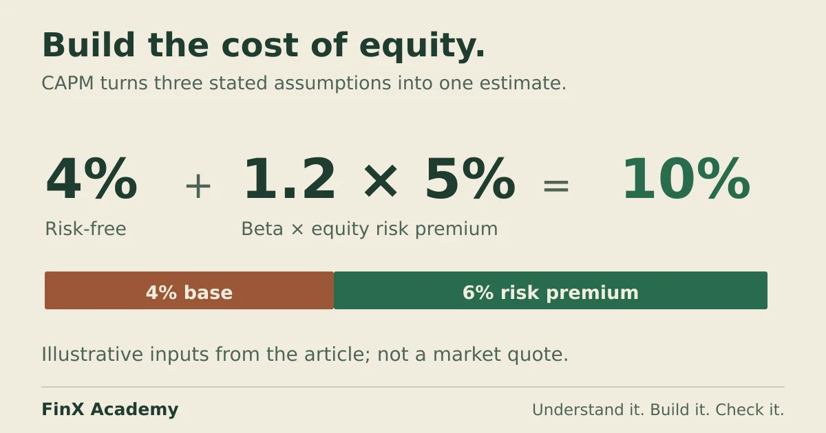
r_e = r_f + β × (E[r_m] − r_f)  =  r_f + β × ERP

• r_f — the time value of money: a dated default-free yield in the same currency as the cash flows, taken at a long maturity because a DCF prices cash flows over decades, not a short T-bill.
• β — a dimensionless multiplier, not a rate: the sensitivity of equity returns to market returns. A regression estimates the slope, not the percentage of price movement explained by the market; that explanatory share is a different statistic, R².
• ERP = E[r_m] − r_f — the equity risk premium: the expected market return above the risk-free rate, per unit of systematic risk, for the part of investing that cannot be diversified away. The model’s logic is exactly that: diversified investors are only compensated for risk they cannot shed, and beta measures the exposure they cannot shed.

Many sources quote the left-hand form with the market return E[r_m] written out. This page stores the premium directly, on the right, because the left-hand form invites the second silent error below: entering a market return into a cell that the formula treats as a premium.

Enter the three assumptions explicitly

Labels in column A, values in column B. This is the same table the WACC build entered at B8–B10; here it is the whole of the workpaper:

Cell	Assumption	Value
B2	Risk-free rate	4.0%
B3	Beta	1.2
B4	Equity risk premium	5.0%

The provenance of each row is the part no template gives you:

• B2 stands for the yield on a long-dated government bond in the cash flows’ currency, taken as of a stated date — in this fiction, 31 August 2026. A real build cites the dated quote and addresses sovereign default risk where a government bond is not a suitable default-free proxy. The choice of horizon matters: matching the rate to the cash flows is why Damodaran’s cost-of-equity chapter walks through the maturity and currency rules, and why a 13-week bill yield is not a drop-in substitute.
• B3 stands for a regression beta — the slope of this stock’s returns against an index, commonly five years of monthly observations. It is a noisy estimate: the result moves with the window and the index chosen. Estimating beta from a peer set is covered in the unlevered-beta guide; on this page 1.2 is an assembled input, the same way the WACC page took the resulting 10.0% as one.
• B4 stands for a published, dated premium survey or an implied-premium estimate; 5.0% is an illustrative assumption, not a current market quote. Damodaran’s project guidance distinguishes historical and implied equity premia. They use different evidence and can produce different answers; state which one you used.

All three are stated guesses, labelled as guesses — which is the honest floor for an exercise page. The deliverable is never just “10%”; it is the range the inputs support and the reason for picking a point inside it.

Assemble the rate

Cell	Row	Formula	Result
B6	Cost of equity (CAPM)	=B2+B3*B4	10.0%

Before reading on: the premium contribution must be exactly 1.2 × 5.0% = 6.0 points, so the answer must be 4.0 + 6.0. Anything else is a wiring error, however confident it looks. Display two decimals and never type a rounded “10%” downstream — the WACC page shows what a 0.37-point rate error does to a terminal value, and a linked rate updates when its assumptions change whereas a typed constant does not.

Audit it: three cheap checks

1. Contribution check. =B3*B4 → 6.0 points must equal =B6-B2 → 6.0 points. The check is mechanical, but it fails loudly when the formula references a different cell than the one you are reading — the most common way a rate “changes without anyone changing it.”
2. Bounds. r_f ≤ r_e, and for beta between 0 and 2, r_e should sit between 4.0% and r_f + 2×ERP = 14.0% here. These bounds require 0 ≤ β ≤ 2 and ERP ≥ 0, with ERP fixed at 5% here. They are scenario checks, not universal market limits. A negative-beta asset can have a CAPM return below the risk-free rate, as Damodaran’s concept check explains.
3. Market-line anchor. A β of 1.0 must return r_f + ERP = 9.0% — the market itself. Northgate’s 1.2 must beat that anchor by exactly (β − 1) × ERP = 1.0 point → 10.0% ✓. This check catches whole families of mistakes at a glance because the gap has an exact, named size.

What no audit catches: an input that is a bad guess on its own terms. The checks verify the arithmetic; the provenance bullets verify the inputs. Both are required, which is the same division of labour the WACC audit uses.

The units error: a 604% cost of equity

To reproduce this error, enter 5 in a General-format B4, then apply Percentage format. Its stored value remains 5, displayed as 500%. With B2 storing 0.04 and B3 storing 1.2, the unchanged formula returns:

r_e = 0.04 + 1.2 × 5.00 = 6.04  →  displays 604.0%

Microsoft documents different entry behavior for an already percent-formatted empty cell: typing 5 there can produce 5%, not 500%. The order above matters. Imported values or formulas storing 5 still represent 500% when displayed as a percentage. Two habits keep a scale mismatch out: enter rates with the percent sign (5%, which stores 0.05), and hold one scale per model — percent format is a display choice, not a value, and a cell containing 5.00 holds a 500% rate no matter what it looks like.

Two silent errors: plausible numbers in the wrong term

1. Beta applied to the wrong term. =B2*B3+B4 — multiply the risk-free rate by beta and add the premium — returns 4.0 × 1.2 + 5.0 → 9.8%. It passes every bounds test. The gap has an exact signature: (β − 1) × (ERP − r_f) = 0.2 points — which vanishes at β = 1, the one input your entire model exists to say is not 1. Through to value, at the WACC page’s 70.59% equity weight: WACC falls 0.14 points to 8.02%, the terminal denominator at g = 2% goes 6.16 → 6.02, and the terminal value comes out 2.3% overstated from a formula that “looks like CAPM.”

2. A market return entered as a premium. B4 = 9.0% — the expected market return, not the bracketed E[r_m] − r_f — gives 4.0 + 1.2 × 9.0 = 14.8%, a gap of exactly β × r_f = 4.8 points. The signature is in the inputs, not the answer: the source labels 9.0% as a market return, so first subtract the stated 4.0% risk-free rate to get a 5.0% premium. A 9% premium is not inherently impossible; it is wrong for these inputs.

Neither error produces an impossible number; both produce a different valuation. That is why this page anchors each check to an exact, named gap instead of a shrug.

How wide is the estimate? A sensitivity exercise

Keep the risk-free rate at 4.0% and flex beta and the premium across illustrative ranges. The cell values are r_f + β × ERP:

β \ ERP	3%	4%	5%	6%	7%
0.8	6.4%	7.2%	8.0%	8.8%	9.6%
1.0	7.0%	8.0%	9.0%	10.0%	11.0%
1.2	7.6%	8.8%	10.0%	11.2%	12.4%
1.4	8.2%	9.6%	11.0%	12.4%	13.8%
1.6	8.8%	10.4%	12.0%	13.6%	15.2%

The risk-free rate moves every cell one-for-one: at rf = 3.5% or 4.5%, the whole table shifts ∓0.5 points. Read what that means for a valuation. Even holding beta fixed at 1.2, one point of premium is 1.2 points of r_e, and at the WACC page’s equity weight it is ±0.85 points of WACC; the terminal-value guide owns the perpetuity mechanics, but the arithmetic is unavoidable — the 6.16-point denominator at g = 2% becomes 5.31 or 7.01, and the terminal value moves +16% / −12%, asymmetrically, because the denominator is small and convex. The corner-to-corner spread of this illustrative table is nearly nine points of required return. A DCF that quotes a point estimate from CAPM without its table is quoting false precision.

When CAPM is the wrong tool

• It prices only systematic risk. A diversified marginal investor is not paid for company-specific exposure — but the founder, the employee and the private-business owner are concentrated. Build-up estimates for private and small companies add size and company-specific premia on top; those add-ons are opinions, so give each one a source and treat the total as a range, not a rate.
• History is not expectation. Beta is a regression on past co-movement with an index; the relationship drifts, and a levered recapitalisation changes a company’s equity beta outright. The peer-based unlever/relever discipline exists precisely because a single regression line is a fragile summary of forward risk.
• It is one factor. Empirically, returns load on size, profitability and other variables CAPM omits; the model survives in practice because it is simple, auditable and defensible — not because it explains realized returns.
• A dividend alternative answers a different question. r_e = D1/P0 + g works only for steady payers — Northgate’s articles declare no dividend, deliberately. For a stable payer priced at 24.00 with D1 of 1.20 and 2% growth, it implies 5.0% + 2.0% = 7.0%: the return the market price already embeds, not a required return derived from risk. When these illustrative methods disagree — 7.0% vs 10.0% here — you have learned something about the assumptions, which is more than either number alone. (Use D1, next year’s dividend. If D0 were 1.20 instead, D1 would be 1.224 and the implied return would be 7.10%.)
• And the ground rule: the cost of equity is what investors require, not what the company pays. Revised return expectations can affect the share price; they do not create a payment obligation. Treating r_e as an expense line is the deepest category error in the whole topic.

Check your answers

• Assembly: contribution 1.2 × 5.0% = 6.0 points; r_e = 4.0 + 6.0 = 10.0%.
• Checks: B3*B4 = B6-B2 ✓; bounds 4.0% ≤ 10.0% ≤ 14.0% ✓; market line 9.0% + (β−1)×ERP = 1.0 pt ✓.
• Units error: 5 entered in General, then formatted as Percentage → 5.00 stored → r_e = 6.04 → 604.0%.
• Silent errors: beta on the wrong term → 9.8%, gap (β−1)×(ERP−r_f) = 0.2 pt, TV 2.3% overstated; market return as premium → 14.8%, gap β×r_f = 4.8 pts.
• Sensitivity: table spans 6.4%–15.2%; at β = 1.2, ±1 pt of ERP → ±1.2 pt of r_e → ±0.85 pt of WACC → terminal value +16% / −12%.

Take the next step

The assembled rate feeds the WACC build, which owns the capital weights, the tax shield and the discount-rate audit, and the DCF guide discounts the cash flows with it; the terminal-value guide shows why every input on this page matters most in the perpetuity denominator. FinX’s Financial Modeling & Valuation course includes DCF practice with paid access — browse the catalogue for the current lessons. The free ten-minute diagnostic asks five numeric modelling questions; it does not grade a cost of capital.