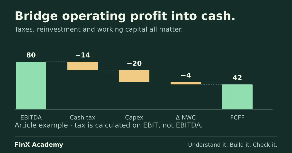
Unlevered free cash flow: bridge EBITDA to cash

Unlevered free cash flow (also called free cash flow to the firm, FCFF) is the cash the operating business generates for all of its capital providers — debt and equity together — after operating taxes calculated before the interest tax shield, reinvestment and working-capital needs, and before any interest or debt repayment. “Unlevered” does not mean “after paying the bank”; it means the number is deliberately computed as if there were no bank. That is what lets you value it with a WACC-based method such as the DCF model example, which discounts exactly this quantity.

The confusion this page untangles is the starting point: analysts are handed an EBITDA and asked for a cash flow. EBITDA is an earnings measure, not free cash flow. The bridge below walks Northgate Logistics’ fictional Year 1 from the first figure to the second, reconciles it a second way, and separates the levered number that often gets confused with it. Amounts are in millions of one currency. This is a new forecast case for Northgate; its operating inputs are supplied below.

Why “unlevered” and why it matters

Northgate’s debt claims sit ahead of its shareholders. Interest and principal payments move cash between the business and its lenders, but they do not change what the operations produce. Unlevered free cash flow excludes those financing movements so that the operating business can be valued independently of how it is funded — the same pairing logic behind enterprise value versus equity value: a value for all providers goes with cash flow to all providers, discounted at a blended cost of capital (assemble and audit one here). Damodaran’s NYU Stern lecture on discounting cash flows sets out that matching requirement; the DCF guide cites the same source.

EBITDA is the natural starting point for the bridge because it already sits at the operating level — but it stops short of cash twice over: it deducts nothing for tax or reinvestment, and it hasn’t touched working capital at all.

Set up the Year 1 forecast

Enter these fictional inputs in a blank sheet, label in column A, value in column B:

Cell	Input	Value
B2	Revenue	400.0
B3	EBITDA	80.0
B4	Depreciation and amortisation	24.0
B5	Operating cash tax rate	25%
B6	Capital expenditure	20.0
B7	Increase in operating working capital	4.0

The tax assumption is deliberately simple: one cash rate on operating profit, with book D&A assumed fully deductible for tax in the same period and sufficient taxable profit to use the deduction. Real tax provision involves filings, rates, shields and timing that a single-line bridge cannot model — state whatever assumption you use. Capex and the working-capital increase are entered as positive uses of cash; the bridge subtracts them, the same convention the DCF build uses. The working-capital line is the cash cost of growth — the working-capital schedule guide explains how to derive an increase from receivables, inventory and payables in a separate example. The 4.0 here is a supplied input. The 24.0 charge and 20.0 capex are supplied inputs here; the depreciation schedule guide builds the PP&E schedule for the same Northgate Year 1 from an opening asset base and derives exactly these two figures.

Before reading on, predict the answer: starting from EBITDA of 80, is Year 1 unlevered free cash flow closer to 60, to 42, or to 20? The arithmetic decides; the bridge says which items move it and why.

Build the bridge line by line

Cell	Row	Formula	Result
B10	EBITDA	=B3	80.0
B11	Operating profit (EBIT)	=B10-B4	56.0
B12	less cash tax on EBIT	=-B11*B5	−14.0
B13	After-tax operating profit (NOPAT)	=B11+B12	42.0
B14	add back D&A (non-cash)	=B4	24.0
B15	less capital expenditure	=-B6	−20.0
B16	less increase in operating working capital	=-B7	−4.0
B17	Unlevered free cash flow	=SUM(B13:B16)	42.0

Each step exists because EBITDA skipped it:

• D&A out, tax on EBIT, D&A back in. Subtract 24.0 to move from EBITDA to EBIT, then add it back after calculating operating tax because it is a non-cash expense. Those two entries cancel before tax; under the stated deduction assumption, D&A still reduces tax by 24 × 25% = 6.0. That tax saving is its net contribution to this bridge.
• Operating tax. 14.0 is the unlevered tax assumption, before any interest tax shield. The actual cash tax bill of an indebted company can differ; the financing example below gives 11.5 when interest is deductible.
• Capex. EBITDA ignores reinvestment entirely; a business spending 20.0 to stand still has 20.0 less cash.
• Working capital. Growing revenue by this plan absorbed 4.0 into receivables and inventory beyond payables.

The result, 42.0, is what the operating business generated for all providers. The DCF guide’s one-line formula, EBIT × (1 − tax) + D&A − capex − ΔOWC, is this same bridge compressed: 56 × 0.75 + 24 − 20 − 4 = 42.

Cross-check with the shortcut

Bridge from EBITDA without ever visiting EBIT, taxing the EBITDA directly and adding back the tax shield D&A would have created:

EBITDA × (1 − t) + t × D&A − capex − ΔOWC
= 80 × 0.75 + 0.25 × 24 − 20 − 4
= 60 + 6 − 24 = 42.0

Same answer, arrived at independently — the kind of two-route check that catches a transposed sign somewhere above. If the routes disagree, the difference equals the item one of them mishandled; here the t × D&A = 6.0 term is exactly the shield computed in the long bridge.

Levered is a different question

Once the operations have produced 42.0, the financing claims get paid from it. Suppose Northgate carries 200.0 of debt outstanding for the full year at a 5% cash rate, with no fees or capitalised interest: interest of 10.0, fully tax-deductible at 25%, costs the equity holders 7.5 of after-tax cash, before any principal repayment or new borrowing. Cash flow available to equity is therefore around 42.0 − 7.5 = 34.5 (plus borrowings, minus repayments) — a number paired with the cost of equity and equity value, never with a WACC. The actual tax bill in this simplified levered case is (56 − 10) × 25% = 11.5, compared with 14.0 before the interest shield. The debt-schedule guide demonstrates opening-balance interest and payment timing on a different loan; its interest figures are 8.0, 9.6 and 7.2.

Three ways the bridge goes wrong

1. EBITDA − capex and calling it cash flow. Here that is 80 − 20 = 60 — overstating the answer by exactly 18, which is the 14.0 cash tax plus the 4.0 working-capital build. The D&A subtraction people worry about actually cancels in this shortcut, which is why the error looks so plausible: it fails only on the two cash items EBITDA never mentions.

2. Forgetting the D&A add-back. Compute NOPAT, subtract capex and working capital, and the bridge lands at 42 − 20 − 4 = 18 — understated by exactly 24, the non-cash depreciation and amortisation deducted when calculating EBIT. The signature is the difference matching the D&A line: when an error’s size equals a specific row, audit that row’s direction.

3. Subtracting interest “for safety.” Deduct the 10.0 here and you get 32.0, then discounting at WACC adds a second charge for the same debt: the rate already pays lenders their required return. The interest belongs in the levered figure (34.5 above), not in the unlevered bridge. This is a pairing mistake, the same one this series keeps meeting from different directions — see the classification discipline in the valuation-bridge article.

Check your answers

• EBIT 56.0; cash tax 14.0; NOPAT 42.0; unlevered FCF 42.0 (=SUM(B13:B16)).
• Shortcut: 60 + 6 − 24 = 42.0; the shield term equals t × D&A = 6.0.
• Error 1: 60.0, overstated by 18.0 = tax 14.0 + ΔOWC 4.0.
• Error 2: 18.0, understated by 24.0 = D&A.
• Interest 10.0; after-tax cost 7.5; levered cash flow to equity 34.5 before principal movements — and 32.0 is a double count, not a conservative estimate.

Take the next step

This type of cash flow is what the DCF model example forecasts on a different dataset for five years, discounts and bridges to equity value; the three-statement model guide shows which income and balance-sheet lines feed each row of the bridge. FinX’s Financial Modeling & Valuation course includes DCF practice with paid access — browse the catalogue for the current lessons. The free ten-minute diagnostic asks five numeric modelling questions; it is not a cash-flow assessment and does not grade this bridge.