Depreciation schedule in Excel: connect capex, depreciation and net PP&E

A depreciation schedule answers two questions for property, plant and equipment (PP&E): what is the depreciation expense for each period, and what net book value closes on the balance sheet? It is a roll-forward in the same shape as a debt schedule: open the balances, add the period’s movements, close the balances, and keep the timing convention visible.

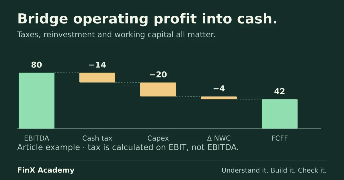
This page builds a three-year schedule for Northgate Logistics, the fictional company used in the unlevered free cash flow bridge. That article supplied Year 1 depreciation and amortisation of 24.0 and capital expenditure of 20.0 as inputs; here the same two figures are derived from an asset base, so the charge and the balance agree with each other instead of being asserted. We treat Northgate’s assets as tangible, so this depreciation is the whole D&A line. Amounts are in millions of one currency. No download is advertised; the tables below are the complete model, with cell addresses, so you can rebuild and extend it.

Decide the convention before the formula

Straight-line depreciation needs decisions before any Excel formula:

• Depreciate cost, not book value. A straight-line charge is cost divided by useful life (salvage value, if any, is subtracted first). This example assumes zero salvage.
• Choose a convention for additions. Here, assets bought during a year take a full year of depreciation in the year of purchase. A half-year convention would instead charge half the annual amount, changing Year 1 from 24.0 to 22.0 — a different model, not a different formula.
• Stop the charge at the end of the life. A cohort depreciates for exactly its life and then charges zero.

Excel has built-in functions for single assets, but they do not build a schedule on their own. SLN(cost, salvage, life) returns the constant per-period amount for one asset and has no period argument, so copying it along a timeline never starts or stops a cohort by itself (Microsoft’s SLN documentation). The standard alternative is an explicit cohort table guarded by IF conditions on the year — exactly what ICAEW’s depreciation-schedule guide recommends for the same reason. Declining-balance and units-of-production methods are different conventions entirely; this page keeps to the straight-line basics.

Disposals are deliberately out of scope. When an asset is sold, its cost leaves the gross roll-forward and its accumulated depreciation leaves the accumulated roll-forward; add that machinery only once the simple schedule reconciles.

Enter the inputs

Label in column A, values in column B:

Cell	Input	Value
B2	Cost of the existing fleet	200.0
B3	Useful life of the existing fleet (years)	10
B4	Years of that life already taken before Year 1	3
B5	Capital expenditure in each of Years 1–3	20.0
B6	Useful life of new assets (years)	5

Four quantities follow from these inputs. The existing fleet charges =B2/B3 = 20.0 a year and has already accumulated =B2/B3*B4 = 60.0, so it opens the schedule at a net book value of 200.0 − 60.0 = 140.0. Each capex cohort charges =B5/B6 = 4.0 a year for five years.

Build the depreciation charge by cohort

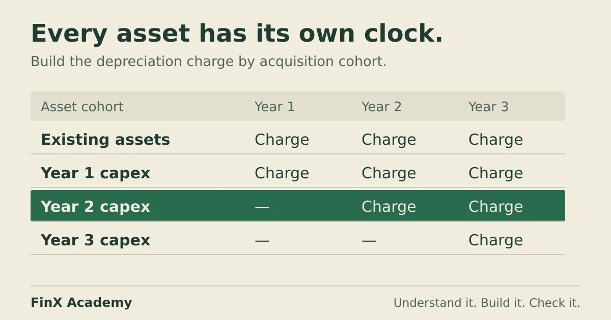
Use columns C:E for Years 1–3. Each row is one cohort of assets; a cohort charges nothing before its purchase year. Before reading the totals, predict them: does the expense grow across the three years, and by how much per new cohort?

Row	Cohort	Year 1	Year 2	Year 3
9	Existing fleet	20.0	20.0	20.0
10	Year 1 additions	4.0	4.0	4.0
11	Year 2 additions	0.0	4.0	4.0
12	Year 3 additions	0.0	0.0	4.0
13	Depreciation expense	24.0	28.0	32.0

Enter =$B$2/$B$3 in C9 and copy across. Enter =$B$5/$B$6 in C10 and copy across; in row 11 leave C11 at zero and enter the same formula in D11:E11; in row 12, zero through D12 and the formula in E12. In C13, enter =SUM(C9:C12) and copy across.

The rising expense is not an error: the fleet is growing, and every cohort from its purchase year onwards adds its 4.0 until its own five-year life ends. In this three-year window no cohort ever stops, which is why the copy-down above is safe. Over a longer horizon you would guard each cell on both boundaries — charge only while the year index is at or after the purchase year and before the purchase year plus the life — rather than letting a filled formula run past the end of an asset’s life.

Roll forward gross, accumulated and net

Row	Roll-forward	Year 1	Year 2	Year 3
16	Gross PP&E, opening	200.0	220.0	240.0
17	Additions (capex)	20.0	20.0	20.0
18	Gross PP&E, closing	220.0	240.0	260.0
19	Accumulated depreciation, opening	60.0	84.0	112.0
20	Depreciation expense	24.0	28.0	32.0
21	Accumulated depreciation, closing	84.0	112.0	144.0
22	Net PP&E, closing	136.0	128.0	116.0

In C16 enter =$B$2 (opening gross) and in C19 =$B$2/$B$3*$B$4 (opening accumulated). Enter the movements in C17 (=$B$5) and C20 (=C13), then the closes =C16+C17 in C18, =C19+C20 in C21 and =C18-C21 in C22. Carry each close into the next opening — D16 =C18 and D19 =C21 — and copy the formula rows across to Year 3.

Two checks should now agree from different directions:

1. Net roll-forward. Closing net equals opening net plus capex minus the charge: 140.0 + 20.0 − 24.0 = 136.0, then 136.0 + 20.0 − 28.0 = 128.0, then 128.0 + 20.0 − 32.0 = 116.0.
2. Independent accumulated balance. Age every cohort at Year 3: the existing fleet has taken 3 + 3 = 6 years at 20.0, and the cohorts have taken 3, 2 and 1 years at 4.0: 6 × 20.0 + (3 + 2 + 1) × 4.0 = 144.0. Closing net is then 260.0 − 144.0 = 116.0, matching row 22.

The Year 1 charge of 24.0 and additions of 20.0 are exactly the figures the unlevered cash-flow bridge took on trust. Net PP&E falls over all three years because each year’s charge (24.0 rising to 32.0) exceeds that year’s capex (20.0). The existing fleet’s 20.0 charge exactly matches the 20.0 of capex, so the whole decline — 4.0, then 8.0, then 12.0 — is the charge on the new cohorts themselves. The balance would flatten only if additions rose to match the total charge.

Where the rows go in the model

Schedule row	Destination
Depreciation expense (row 13)	Income statement, within operating costs
Depreciation expense, added back; capex as an outflow	Cash flow statement (indirect operating section; investing section)
Net PP&E, closing (row 22)	Balance sheet, non-current assets

The SEC’s introduction to financial statements explains why the expense and the cash flow are presented separately. The three-statement example shows what a missing depreciation add-back does to the balance check; this schedule is the supporting detail behind that line (three-statement model).

Check an input change flows through

Change Year 2 capex from 20.0 to 30.0. The Year 2 cohort now charges =30/5 = 6.0 a year from Year 2. Expected results: depreciation 24.0, 30.0 and 34.0; closing net PP&E 136.0, 136.0 and 122.0. Gross closes at 220.0, 250.0 and 270.0; accumulated at 148.0. If Year 3 does not move at all, the schedule is not carrying its balances forward — the same failure the debt-schedule input-change check is designed to catch.

Three ways this schedule goes wrong

1. Additions start depreciating the year after purchase. Drop row 10’s Year 1 cell to zero and the charge falls to 20.0 — understated by exactly 4.0, the first-year cohort charge, with closing net PP&E overstated by the same amount. Nothing crashes; the convention simply differs from the one stated. The signature is a gap equal to one cohort-year.

2. Depreciate opening net book value over the original life. 140 ÷ 10 = 14.0 plus the 4.0 cohort gives 18.0 — understated by 6.0. Straight-line divides cost by original life. Book value has already had three years taken off, so it must be spread over the remaining seven years: 140 ÷ 7 = 20.0 gives the same charge as cost over original life. Mixing a reduced base with the full life undercharges every year. This error keeps the roll-forward internally consistent, because the roll consumes the same wrong number; only an independent check, like the cohort-age calculation above, exposes it.

3. Capex is missing from the gross roll-forward while the cohort table still charges depreciation. In Year 1, closing gross stays at 200.0 and closing net prints 116.0, but the net roll-forward says 136.0. The 20.0 difference is exactly the omitted capex line — when a check’s difference equals a specific row, audit that row.

Check your answers

• Derived inputs: existing charge 20.0/year; opening accumulated 60.0; opening net 140.0; cohort charge 4.0/year.
• Depreciation expense: 24.0, 28.0, 32.0 (=SUM(C9:C12)).
• Closing gross 220.0 / 240.0 / 260.0; closing accumulated 84.0 / 112.0 / 144.0; closing net 136.0 / 128.0 / 116.0.
• Input change (Year 2 capex 30.0): charge 24.0 / 30.0 / 34.0; net 136.0 / 136.0 / 122.0.
• Half-year convention instead: Year 1 charge 22.0.
• Errors: 4.0 = missing first cohort-year; 6.0 = book value over cost life; 20.0 = capex omitted from gross.

Take the next step

The same roll-forward discipline drives the debt schedule (principal, repayments and interest timing) and the working-capital schedule (receivables, inventory and payables), and the charge built here feeds the unlevered cash-flow bridge and the three-statement model. FinX’s Three-Statement Build course covers supporting schedules; browse the catalogue for the current syllabus and access requirements. The free ten-minute diagnostic asks five numeric modelling questions; it does not grade a workbook schedule.