Working capital schedule: forecast receivables, inventory and payables

A working-capital schedule forecasts receivables, inventory and payables, then reports the change in the total as a cash-flow effect. It converts balance-sheet items into an input the cash-flow statement and the DCF model can use: growth in operating working capital absorbs cash, and a decline releases it.

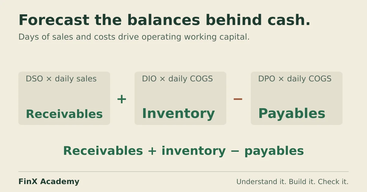
Each balance is forecast from a driver — days sales outstanding (DSO), days inventory outstanding (DIO) or days payable outstanding (DPO) — rather than guessed as a percentage growth rate. The driver is the assumption you defend; the balance is its output. (The same three drivers also condense into one speed metric read backwards from the statements — the cash conversion cycle works that measurement and converts its days into cash.)

Separate operating from total net working capital

The general formula is:

Net working capital = Current assets − Current liabilities

That total measure includes cash and short-term debt, which this model handles separately. For this simplified business, operating (non-cash) working capital is receivables plus inventory minus payables. A fuller model may include other operating balances, such as prepayments, accrued expenses and deferred revenue. Excluding cash avoids double counting, because the cash the business generates is exactly what the schedule helps explain. The SEC’s introduction to financial statements describes how current assets and current liabilities are classified on the balance sheet.

The two measures reconcile directly. At the end of Year 1 in the example below, assume the fictional business also holds cash of 80 and short-term debt of 40:

Year 1 measure	Amount
Current assets: cash 80 + receivables 187.5 + inventory 150	417.5
Current liabilities: payables 75 + short-term debt 40	115
Net working capital: 417.5 − 115	302.5
Operating working capital: (417.5 − 80) − (115 − 40)	262.5

The 262.5 operating figure equals the schedule total you will build. Cash and short-term debt cancel out of the operating measure.

Set the drivers and the forecast inputs

Use a blank worksheet. All figures are fictional, in millions of one currency. Year 0 is the last historical year; Years 1–3 are forecasts. The example uses a 360-day year, a common simplifying convention; state whichever convention your model uses and apply it consistently.

Enter the drivers once, so every year reads them from the same cells:

Cell	Driver	Input
B2	Days in the year	360
B3	DSO — days to collect receivables	45
B4	DIO — days of inventory held	60
B5	DPO — days to pay suppliers	30
B6	Cost of goods sold as a share of revenue	60%

Use columns B–E for Year 0 through Year 3. Enter the revenue history and forecast as inputs in row 8, and calculate COGS in row 9:

Row	Label	B: Year 0	C: Year 1	D: Year 2	E: Year 3
8	Revenue	1,200	1,500	1,800	2,100
9	COGS	720	900	1,080	1,260

The formula in B9 is =B8*$B$6, copied across to E9. The dollar signs hold the driver fixed while the revenue reference moves; the absolute-reference guide explains this pattern.

Build the three-year schedule

Each balance equals its driver divided by the day count, multiplied by the flow it relates to. Assume all sales are on credit, and use COGS as a proxy for credit purchases when forecasting payables. If purchases differ materially from COGS, model those purchases separately and define DPO on that basis. Inventory uses COGS, rather than the selling price.

The drivers here are defined against closing balances. Historical days ratios often use average balances; do not mix those definitions when choosing forecast assumptions. Enter these formulas in column B and copy each across to E:

Row	Label	Formula in B	Year 0 result
11	Receivables	=B8*$B$3/$B$2	150
12	Inventory	=B9*$B$4/$B$2	120
13	Payables	=B9*$B$5/$B$2	60
14	Operating working capital	=B11+B12-B13	210

The completed schedule:

Row	Label	Year 0	Year 1	Year 2	Year 3
11	Receivables	150	187.5	225	262.5
12	Inventory	120	150	180	210
13	Payables	60	75	90	105
14	Operating working capital	210	262.5	315	367.5
16	Increase in operating WC	—	52.5	52.5	52.5

Row 16 starts in column C, because a change needs a prior year: =C14-B14, copied to E16. Year 0 has no increase — keep the cell empty rather than entering zero, so nobody mistakes a missing calculation for a real one.

The increase is constant here because revenue grows by a constant 300 each year. Decompose Year 1 to see the mechanics: receivables rise 37.5, inventory rises 30, and payables rise 15. The payables increase is a source of cash, so it nets against the other two: 37.5 + 30 − 15 = 52.5 absorbed. Real forecasts rarely stay constant; when DSO improves or inventory days stretch, this schedule shows exactly which year the cash effect lands in.

Take the sign of the change once, deliberately

An increase in operating working capital is a use of cash. The business funded 52.5 more receivables and inventory than it deferred through payables; that money is tied up, not available. A decrease is a source: collections outran purchases and cash came back.

In the free-cash-flow formula the sign appears as a subtraction:

FCFF = EBIT × (1 − tax rate) + D&A − capex − increase in operating working capital

This matches the DCF model example, where the working-capital increase is entered as a positive number in row 10 and subtracted in the FCFF formula. Whichever layout you use, the increase must reduce cash flow exactly once. If your schedule outputs the cash-flow effect directly, negate it in the schedule: =-C16 gives −52.5, and the cash-flow statement adds that value without a second sign change.

Catch a payables forecast on the wrong base

A realistic error: building payables on revenue instead of COGS. Change B13 to =B8*$B$5/$B$2 and copy across:

Row	Correct (COGS base)	Wrong (revenue base)
Payables, Year 1	75	125
Operating WC, Year 0	210	170
Operating WC, Year 1	262.5	212.5
Increase per year	52.5	42.5

Every result still looks plausible. The schedule understates the cash absorbed each year by 10, and in a valuation that error compounds across the forecast and into terminal value.

The check that exposes it converts each balance back into days and compares it with the driver. In an empty cell calculate implied DPO for Year 1:

=C13/C9*$B$2

With the correct formula this returns 30, matching B5. With the revenue-based formula, C13 is 125 and COGS is 900, so it returns 50 — the schedule no longer means what the driver cell says it means. Run the same check on the other two balances:

Implied check	Formula (Year 1)	Expected
DSO	=C11/C8*$B$2	45
DIO	=C12/C9*$B$2	60
DPO	=C13/C9*$B$2	30

Copy the three checks across Years 2–3; every result should equal its driver cell. Restore B13 to =B9*$B$5/$B$2 and copy it across through E13 before continuing. Confirm that all four payables balances and all three forecast DPO checks return to their correct values.

Two further failure modes deserve a mention. A sign flip — adding the increase instead of subtracting it — overstates each year’s cash flow by 105 in this example, 315 across the three forecast years, before any discounting. If a missing Year 0 balance is treated as zero, the Year 1 “increase” becomes the full closing balance of 262.5 instead of 52.5. Keep the historical column in the schedule so every change has a base.

Check the schedule before it feeds the model

Before connecting the schedule to a cash-flow statement:

1. Each implied-days check equals its driver cell in every forecast year.
2. The Year 0 balances reconcile to the historical balance sheet, not just to the formulas.
3. The increase row is empty — not zero — in Year 0.
4. The sign convention is applied exactly once, in the schedule or in the cash-flow statement.

When the schedule feeds a full model, the closing receivables, inventory and payables balances must also appear on the forecast balance sheet, and the cash effect must appear in the cash-flow statement. If total assets and liabilities then disagree, the balance-sheet troubleshooting example shows how to isolate the broken link rather than forcing the difference to zero.

Take the next practice step

This schedule is one supporting schedule in a connected model. The three-statement guide shows how receivables, inventory and payables balances flow into the balance sheet, and the debt schedule builds the financing side with the same forecast-and-check discipline.

FinX’s Three-Statement Build course includes a paid working-capital lesson where you build DSO, DIO and DPO drivers into one integrated model; browse the course catalogue for the current syllabus and access requirements. For a short free starting point, try the modelling diagnostic: five questions in ten minutes, checking selected skills rather than a full model build.