Build a debt schedule: connect repayments, interest and closing debt

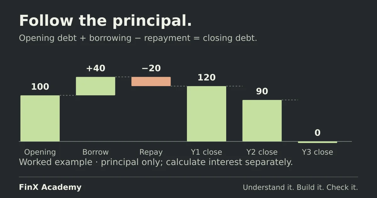
A debt schedule explains how borrowing changes over time. It starts with opening principal, adds new borrowing, subtracts principal repayments and calculates closing debt. Interest needs its own calculation because the balance outstanding during a period can differ from the balance at its end.

Start with one borrowing facility and explicit assumptions. You can add other facilities after each individual schedule reconciles.

Separate principal from interest

Principal is the amount borrowed that remains outstanding. A cash interest payment pays for borrowing during a period; in the simple cash-pay loan below, it does not reduce principal.

The schedule has three connections to a financial model:

Schedule item	Connection
Closing principal	Debt on the balance sheet
New borrowing and principal repayment	Financing cash movements
Interest	Interest expense and its corresponding payment or accrual

The SEC’s introduction to financial statements explains that borrowing provides financing cash and loan repayment uses financing cash. The presentation of interest requires the appropriate accounting treatment; keep its calculation separate from principal movements.

Set assumptions that make timing visible

Use this fictional example, in consistent illustrative currency units:

• Opening principal is 100.
• The annual cash interest rate is 8%.
• New borrowing is 40 in Year 1, then zero.
• Planned principal repayments are 20, 30 and 120.
• All borrowing and repayments occur at each year-end, after that year’s interest has accrued. Interest is paid at year-end.
• The business has sufficient cash to make the payments. There are no fees, capitalised interest, discounts or other debt movements.

Planned repayments are inputs to this exercise. Actual repayments are capped at outstanding principal, so the final planned amount cannot create a negative debt balance. A real schedule must also reflect the agreement’s terms and the business’s cash availability.

Build the three-year principal schedule

Put the rate in B2 as 8%. Use columns C:E for Years 1–3 and these row labels in column A:

Row	Label	Year 1	Year 2	Year 3
4	Opening principal	100	120	90
5	New borrowing	40	0	0
6	Planned repayment	20	30	120
7	Actual principal repayment	20	30	90
8	Closing principal	120	90	0
10	Cash interest	8	9.6	7.2
11	Net financing cash from principal	20	−30	−90

Enter the opening principal in C4. Enter borrowing and planned repayment inputs in rows 5 and 6. In C7, cap the repayment at the principal available:

=MIN(C4+C5,C6)

In C8, calculate closing principal:

=C4+C5-C7

Set D4 to =C8, then copy it across to E4. Copy the formulas in rows 7 and 8 across to Year 3. Inputs are assumed non-negative; flag an invalid negative borrowing or repayment input instead of treating it as a legitimate plan.

Year 3 opens with 90. Although the planned repayment is 120, the actual principal payment is 90 and closing debt is zero. The excess planned amount of 30 is not a further principal payment. Without the cap, the schedule would show debt of −30.

Calculate interest for the stated timing

Because principal movements occur at year-end, the opening balance remains outstanding throughout the year in this simplified model. In C10, enter:

=C4*$B$2

Copy across. Interest is 8, 9.6 and 7.2. Year 3 still incurs interest even though closing debt is zero: the 90 opening balance was outstanding during the year.

Using closing debt would incorrectly give zero Year 3 interest. Using the average of opening and closing debt would give (90 + 0) ÷ 2 × 8% = 3.6, which also does not match this example’s year-end repayment assumption.

Average balances can be an approximation when the timing of movements supports them. If dates matter, divide the period into intervals with the relevant balances and apply the agreement’s rate and day-count convention. Decide the timing method before choosing the formula.

Connect the cash flows and check the result

In C11, enter =C5-C7 and copy across. This shows cash received or paid from principal movements. Interest is excluded from this row so that principal repayment and borrowing costs remain distinct.

Check the cumulative reconciliation independently:

Opening principal + total borrowing − total principal repaid
= 100 + 40 − (20 + 30 + 90)
= 0 closing principal

Compare each year’s closing principal with the debt amount linked into the balance sheet. Compare its borrowing and repayment with the financing cash-flow lines. Matching an internally calculated check to itself cannot detect a broken link into another statement.

Now change Year 2’s planned repayment from 30 to 50. Year 2 closing debt should fall from 90 to 70; Year 3 opening debt and final principal payment should also become 70. Year 2 interest stays at 9.6 under the year-end timing assumption, while Year 3 interest falls to 5.6.

This input-change check catches a schedule that calculates the first year correctly but fails to carry the result forward.

Add detail only when the example requires it

With several facilities, give each its own terms, balance movements and interest calculation, then sum the results. A revolving facility or cash sweep may depend on available cash; that is additional logic rather than a reason to force the simple schedule to balance with an unexplained borrowing amount. The circular-reference guide traces an interest-and-borrowing loop and compares timing, algebra and iteration.

The cash-interest row is also the denominator of a ratio: the interest coverage guide reuses this exact schedule to calculate three years of coverage, and shows how a link to the closing-principal row instead silently changes the answer.

Continue with the three-statement model to connect the schedule, or use the balance-sheet troubleshooting guide to investigate a broken link. FinX’s Three-Statement Build course includes debt-schedule practice; browse the catalogue for current access requirements.

At acquisition closing, the sources and uses example explains where the new debt comes from. Then calculate fixed-charge coverage using the agreement’s stated obligations.