Circular references in Excel: trace the loop before you iterate

A circular reference exists when a formula refers back to its own cell, directly or through a chain of other cells. Microsoft’s canonical example is =D1+D2+D3 entered in D3: the answer depends on the answer. In finance workbooks these come in two kinds, and telling them apart is the whole skill. An accidental loop is a broken formula. An intentional loop — interest that depends on debt that depends on interest — is a modelling decision with real consequences. The first response is to trace the chain and classify it, not to switch on iterative calculation and make the warning go away.

All figures below are fictional and use consistent illustrative units. The recurrence tables are independently calculated examples, not measurements from an Excel session. Microsoft’s circular-reference documentation is the reference for the messages, tools and settings described here (desktop Excel for Microsoft 365 and 2016–2024; tracing commands are limited in the web and mobile apps).

Reproduce an accidental loop

Enter this small departmental budget in a blank sheet:

Cell	Item	Amount
B2	Rent	12,500
B3	Software	4,200
B4	Travel	1,800
B5	Utilities	900

The total belongs in B6. Type it one row too wide — a classic edit after inserting a line item:

=SUM(B2:B6)

With iterative calculation off, Excel detects the circular reference. After the warning, B6 may show 0 or its last calculated value, according to Microsoft. Neither is a valid total here: the formula asks the total to equal itself plus another 19,400, which has no solution. The fix is the formula you meant: =SUM(B2:B5) returns 19,400.

The same loop can hide across several cells — Microsoft’s documented two-cell pattern is =B1+1 in A1 with =A1+1 in B1 — so one arrow is not the diagnosis.

Find the chain without guessing

With more than one formula involved, use the tracing tools rather than reading cells:

1. Watch the status bar: it shows “Circular References” and one cell address. Only the label, with no address, means the loop is on another worksheet.
2. Go to Formulas > Error Checking > Circular References. Select a listed cell address to inspect it. You can also use Ctrl+G on Windows or Control+G on Mac to enter a known address.
3. From there use Trace Precedents and Trace Dependents to walk the chain until it points back where you started.
4. Fix one formula, then repeat until the status bar is clear. Fixing one loop does not clear the others.

Do not rely on a fresh warning for every loop: Microsoft says later circular references in the same session might not show the same dialog. Recheck the status bar and trace the dependencies even if the cell displays a plausible value. A circular formula or a formula that depends on it can also produce other errors.

Now the loop you might want: debt that funds its own interest

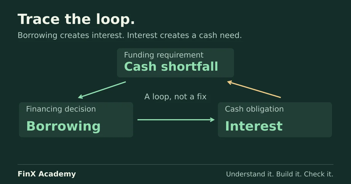
Northgate Logistics, carried over from the enterprise-value bridge exercise, forecasts a Year 1 funding shortfall of 4.5 before revolver interest. Use a separate worksheet from the budget example. Assume no opening revolver debt, all borrowing occurs at the start of the year, the annual rate is 10%, and cash interest is paid at year-end from the borrowed funds. The full borrowing is outstanding all year and includes cash reserved to pay its own interest. So the borrowing B satisfies:

B = 4.5 + 0.10 × B

That is a circular reference by construction: borrowing determines interest, interest determines the cash need, the cash need determines borrowing. With the shortfall in B2 and the rate in B3, entering =B2+B3*B4 in B4 creates an intentional circular reference. Removing the dependency without replacing its economics would understate the funding need.

Pause before calculating: is borrowing of 4.5 enough? No — 4.5 of debt costs 0.45 of interest, which itself needs funding, which adds debt, which adds interest.

Iterate the answer by hand

Excel’s iterative calculation replaces the cell with its own previous result, over and over. You can do the same in a column — no settings required. Start from 0 and compute B_next = 4.5 + 0.10 × B_previous:

Pass	Borrowing B	Change
1	4.50000	4.50000
2	4.95000	0.45000
3	4.99500	0.04500
4	4.99950	0.00450
5	4.99995	0.00045

Each pass changes the answer by one tenth of the previous change, so the sequence approaches 5.0. Applying Excel’s documented default stopping rule — 100 iterations or a change below 0.001 — to this hand calculation stops it at pass 5, at 4.99995 (5.000 to three decimal places). This is an approximation. An actual workbook’s result can differ with its starting values, calculation order and settings; do not assume it will reproduce this exact pass count. Microsoft’s calculation-settings documentation states the trade-off directly: a smaller Maximum Change gives a more accurate result and costs recalculation time.

Three ways to resolve the loop

1. Change the timing convention. The cheapest fix is to remove the simultaneity: calculate interest on the opening balance, with new borrowing assumed to occur at year-end, so current-year borrowing does not incur a full year of interest. That is exactly the choice the debt-schedule guide makes — year-end principal movements, interest on the balance that was outstanding during the year. This changes our start-of-year borrowing assumption: apply it only when year-end timing is appropriate or an explicitly accepted approximation. It removes circularity but would understate interest for the start-of-year draw in this example.

2. Solve it with algebra. For this loop the fixed point is available in closed form:

B = 4.5 / (1 − 0.10) = 5.0        interest = 4.5 × 0.10 / (1 − 0.10) = 0.5

Check: 4.5 + 0.5 = 5.0. Enter these formulas and the workbook is exact with iterative calculation switched off. The cleanup also exposes the model’s real condition: the denominator 1 − rate is positive only while the rate is below 100%. For a positive funding need and a non-negative rate, a finite positive borrowing solution requires 0 ≤ rate < 100%. At 100% there is no solution; above 100% the algebra produces negative borrowing, which cannot fund the stated need, and this iteration diverges.

3. Allow it with iterative calculation. Windows: File > Options > Formulas > Enable iterative calculation; Mac: Excel > Preferences > Calculation > Use iterative calculation. This is the right tool when the loop is too entangled to solve by hand — average-balance interest, cash sweeps, interest that changes the tax bill that changes the cash need. It is the wrong default everywhere else: Microsoft’s guidance is to keep it turned off in most worksheets. Remember that the returned value is a tolerance approximation (4.99995 above), and that results change with the settings — so record the Maximum Iterations and Maximum Change used, and say so in the model notes.

Before accepting any iterative answer, re-substitute it into the loop: compute 4.5 + 0.10 × B and compare with the B displayed. At 4.99995 the mismatch is 0.000045 — the loop has settled. If the mismatch exceeds your acceptance tolerance, the result has not passed the check. Review the iteration limit, tolerances, starting values and the dependency chain; a large residual alone does not prove which setting stopped the calculation.

The failure that iteration hides

Consider the accidental =SUM(B2:B6) in B6 with iteration allowed. The mathematical recurrence adds the 19,400 of costs to the previous total each pass: starting from zero, 19,400 → 38,800 → … → 1,940,000 after 100 passes. Another 100 passes adds 1,940,000 again. These are controlled recurrence results, not guaranteed Excel screen values: cached values and recalculation behavior affect where a live workbook starts and stops. The re-substitution test catches it instantly: the mismatch per pass is the full 19,400, not a rounding dusting.

Enabling iteration can leave an invalid model displaying a number. If you inherit a workbook with iteration enabled, save a copy and record the current settings before changing them. In that copy, turn iteration off to help locate the loops, then classify each as intentional or accidental and verify the replacement formulas.

Check your answers

• Accidental loop: =SUM(B2:B6) in B6 is circular; corrected =SUM(B2:B5) = 19,400.
• Detection: status bar “Circular References” plus a cell address; Formulas > Error Checking > Circular References; later loops may not trigger another warning dialog.
• Revolver loop: hand iteration gives 4.5, 4.95, 4.995, 4.9995, 4.99995 — where the default 0.001 tolerance stops this hand calculation. The exact answers are borrowing 5.0, interest 0.5.
• Closed form B = need/(1 − rate) requires 0 ≤ rate < 100% for a finite positive borrowing solution with a non-negative rate; timing and algebra both work with iteration off.
• Runaway accidental sum under iteration: 1,940,000 after 100 recurrence passes starting at zero = 100 × 19,400; residual check mismatch per pass = 19,400 versus 0.000045 at the converged revolver.

Take the next step

The timing convention used above is practised end to end in the debt-schedule guide, and when a repaired loop still leaves a model inconsistent, the balance-sheet troubleshooting guide traces the break across statements. The three-statement model example makes the same advice this article formalises: build a model you can follow and check before adding circularity. FinX’s Three-Statement Build course includes debt-schedule practice, with later lessons requiring paid access — browse the catalogue for current terms. The free ten-minute diagnostic asks five numeric modelling questions; it does not audit a workbook and is not a substitute for the tracing steps above.