Interest coverage ratio: calculate it and explain what changed

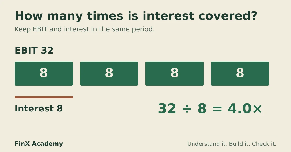
The interest coverage ratio asks how many times a year’s operating profit pays the year’s interest bill:

Interest coverage = EBIT ÷ Interest expense

This EBIT-based measure is also called times interest earned. It measures earnings coverage, not cash available for principal repayments or reinvestment. Damodaran’s NYU Stern corporate-finance materials use this EBIT/interest definition.

It is usually quoted as a multiple — “4.0×” means EBIT could absorb interest four times over. The arithmetic is one division; the analysis is three questions this article works through. Which numerator are you using — EBIT or EBITDA? What changed when the ratio moved? And is the denominator the interest figure your debt schedule actually produces? The example below is a fictional borrower on the same terms as the debt schedule guide, so the final step is a real cross-statement check, not a self-referential one.

Set up the borrower

The company, its facility and its interest figures are fictional, in the illustrative units used by the debt schedule guide: opening principal 100, an 8% annual cash rate, a 40 drawdown at the end of Year 1, and year-end principal movements after the year’s interest has accrued. That schedule — follow it or paste its row — produces cash interest of 8.0, 9.6 and 7.2 for Years 1–3, because interest runs on the opening balance: 100 × 8%, 120 × 8%, 90 × 8%.

For this simple cash-pay loan, interest expense equals cash interest: there are no fees, capitalised interest, payment-in-kind interest or accrual timing differences. A real agreement may require adjustments; reconcile to its defined expense measure instead of assuming cash paid always matches.

The income-statement inputs are new for this exercise: EBIT of 32.0, 36.0 and 28.8, and flat depreciation of 12.0, with no amortisation. On a blank worksheet, put Year 1, Year 2 and Year 3 in C2:E2, the row labels in column A, and enter:

Row	A: Label	C: Year 1	D: Year 2	E: Year 3
4	EBIT	32.0	36.0	28.8
5	Interest expense	8.0	9.6	7.2
7	Depreciation	12.0	12.0	12.0

Calculate the base ratios

In C6 enter the coverage formula and copy it across:

=C4/C5

The answers are 4.00×, 3.75× and 4.00×. Read the middle of that sequence, because it is the part a quoted average hides. EBIT grew from Year 1 to Year 2 — 32.0 to 36.0 is +12.5% — yet coverage fell, because the Year 1 drawdown, net of that year’s 20 repayment, pushed interest up 20% (8.0 to 9.6) in Year 2. Growth and coverage moved in opposite directions. Year 3 closes the same story from the other side: EBIT falls 20% (36.0 to 28.8) while the 30 repayment cuts interest 25% (9.6 to 7.2), and coverage lands back on 4.00× — a stable-looking ratio produced by a profit decline being masked by debt paydown. Same number, different company. That is why an interest coverage answer should name its year and its inputs, not just its level.

Run the same reasoning on the downside. Suppose the Year 3 profit miss is worse: EBIT comes in 25% below the base, at 21.6 (28.8 × 0.75). With interest unchanged at 7.2:

=21.6/7.2

The answer is 3.00×, exactly 25% below the base 4.00× — when only the numerator moves, the ratio carries the same percentage change. Whether 3.0× is comfortable is a question about the lender’s definition and the business’s volatility, not a property of the number itself.

State the numerator convention: EBIT or EBITDA?

Plenty of published coverage figures use EBITDA in the numerator instead of EBIT, and some analysts net interest income against interest expense in the denominator. These are different definitions, so label yours explicitly and use the loan agreement’s definition for a covenant check. They are not interchangeable.

Add EBITDA in A8, Coverage on EBITDA in A9, and enter in C8 and C9, copying across:

=C4+C7
=C8/C5

EBITDA is 44.0, 48.0 and 40.8 (EBIT plus the 12.0 depreciation), and the ratios are 5.50×, 5.00× and 5.67×. The levels are all higher than the EBIT ratios, as they must be — adding back a positive number enlarges the numerator while the denominator is untouched. The subtler cost is that the shape of the story changes: EBIT coverage dipped to 3.75× and recovered to 4.00×, while EBITDA coverage dipped to 5.00× and overshot to 5.67×, because flat depreciation carries a different weight in each year’s mix. Two analysts who correctly run “the coverage ratio” on this borrower can honestly report different trends. The fix is editorial, not mathematical: label the numerator and denominator explicitly.

Reconcile the denominator to the schedule

Here the coverage sheet meets the reason the debt schedule exists. Put Schedule interest in A11, link the three figures from the schedule’s cash-interest row (8.0, 9.6, 7.2), and in A12 build Difference with =C5-C11 across. Every cell must read 0 before the ratio leaves your desk.

Why so strict? Because the denominator is where a broken link shows up as a plausible answer. Reproduce a classic mistake: rebuild the interest row from the schedule’s closing principal row (120, 90, 0) instead of its cash-interest row — 8% on each gives 9.6, 7.2 and 0:

Year	EBIT	Wrong interest	Wrong coverage
1	32.0	9.6	3.33×
2	36.0	7.2	5.00×
3	28.8	0	#DIV/0!

The two surviving ratios are plausible but wrong in opposite directions: Year 1 coverage falls from 4.00× to 3.33× and Year 2 rises from 3.75× to 5.00×, and 9.6 and 7.2 are real numbers in this model — the entire wrong row is the correct row shifted one column. The debt schedule guide warns of exactly this convention error in the schedule itself: with year-end movements, interest belongs to the opening balance, and using the closing balance gives Year 3 a charge of zero even though the 90 balance was outstanding all year. Here the consequence is visible as #DIV/0!: a company that has just repaid its final principal payment is, according to this formula, a company with no interest at all. The Difference row catches all three cases: =C5-C11 returns 1.6, −2.4 and −7.2 against a schedule that independently says 8.0, 9.6 and 7.2.

Change row 5 back to the schedule’s 8.0, 9.6 and 7.2, confirm the Difference row is all zeros, and the base answers return: 4.00×, 3.75×, 4.00×.

When the ratio is uninformative — and what to print instead

Coverage degrades into noise in two regions, and you should notice it before a reader does.

• Interest near zero or negative. A fully repaid borrower earning interest on surplus cash has a net interest income, not expense. With net interest of −1.5 and EBIT of 28.8, the formula returns −19.2×. That negative result reflects net interest income, not an operating loss or evidence of distress. Near-zero positive expense can likewise produce a very large multiple without proving that every other obligation is covered.
• Negative EBIT. EBIT of −2.4 against interest of 7.2 returns −0.33×, and EBIT of −4.8 against 9.6 returns −0.50×. These negative ratios identify operating losses: neither case covers its interest from EBIT. They can still be used in a consistently defined credit screen, but should not be described as a positive number of times interest was covered. Show the loss and interest amounts alongside them.

For this report, show the inputs and flag ratios that need explanation. A minimal guard in C6:

=IF(C5<=0,"n.m.",C4/C5)

returns n.m. (not meaningful) whenever the denominator is zero or negative, and you can nest the EBIT test the same way: =IF(C5<=0,"n.m.",IF(C4<0,"n.m.",C4/C5)). One caveat: the guard’s output is now text for the flagged cells. Microsoft’s AVERAGE documentation explains that text in referenced cells is ignored. =AVERAGE(C6:E6) therefore averages only the numeric ratios and can hide excluded years. Display the flags and inputs; if you need aggregate coverage, define the period and divide total EBIT by total interest for that same period, rather than averaging annual multiples.

Choose the next practice step

Quote coverage as “EBIT of 28.8 against schedule interest of 7.2 — 4.00× in Year 3, 3.00× in the downside”, with the Difference row visible beside it. Then keep the chain going: rebuild the denominator yourself in the debt schedule guide, place the whole borrower inside connected statements with the three-statement model guide, and turn the single downside input into a grid with the sensitivity analysis guide.

FinX’s Three-Statement Build course includes debt-schedule practice, which is where this article’s denominator comes from; browse the catalogue for current syllabus and access requirements, or try the free five-question diagnostic to find the skill to practise next.

To include principal, leases and required cash deductions, compare the defined conventions in fixed-charge coverage.