PMT in Excel: calculate and check a loan payment

PMT, one of Excel’s financial functions, returns the fixed periodic payment that pays off a loan at a constant rate: =PMT(rate, nper, pv), with optional fv (the balance left after the last payment) and type (when payments are due). For a $200,000 loan at 6% repaid in three annual payments it returns −74,821.96, written as (74,821.96) in the currency format Microsoft’s own examples use — the parentheses mean money leaving the business.

The syntax is not where loans go wrong. Two conventions are: PMT only works when rate and nper are in the same period units, and its answer carries a cash-flow sign that has to survive the trip into your model. This article calculates a payment, checks it three independent ways, reconciles each payment into interest and principal, reproduces the classic annual-rate-with-monthly-count mistake and the check that catches it, and pins down the timing and balloon arguments.

Set the loan terms out on the sheet

Use a blank worksheet and a fictional equipment loan, in dollars. Put the labels in column A and the three inputs in column B:

Cell	Label	Value
B2	Principal borrowed	200,000
B3	Annual interest rate	6%
B4	Years of payments	3

Sign convention first, because everything downstream follows it: the loan arrives at closing, so the principal is a positive inflow of 200,000; the payments leave, so PMT will return a negative outflow. The interest rate is the contract rate — fixed, and it applies to the balance still outstanding. Payments fall at each year-end; type defaults to end of period, which is what most schedules assume. PMT’s result includes principal and interest only: Microsoft’s documentation notes it excludes taxes, reserve amounts and loan fees, which belong in their own rows.

Calculate the payment and read its sign

Put Annual payment in A5 and this formula in B5:

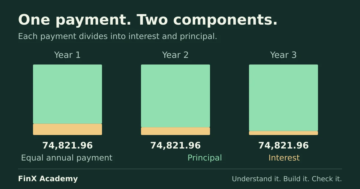
=PMT(B3,B4,B2)

The result is (74,821.96). Why that number: using the full-precision payment, displayed as 74,821.96, at the end of each of three years retires the 200,000 while 6% accrues on the outstanding balance. Every level-payment loan divides the principal by an annuity factor for the rate and term — 2.673012 here, so 200,000 ÷ 2.673012 = 74,821.96 — and PMT computes the factor for you.

If a model needs the payment as a positive size — a display cell or comparison column — use =-PMT(B3,B4,B2). The alternative =PMT(B3,B4,-B2) is also a valid way to calculate a positive payment amount. The important point is consistency: this exercise keeps borrowing positive and the PMT result negative, then negates that result where the schedule displays positive repayment amounts.

Check the payment against the loan

A payment number is cheap to verify because the check is discounting itself — money today equals money later divided by (1 + rate), the same arithmetic behind the NPV function. Add two check rows:

Cell	Label / formula	Result
A6	Check: principal implied by the payment
B6	=PV(B3,B4,B5)	200,000.00
A7	Check: balance after all three payments
B7	=FV(B3,B4,B5,B2)	0.00

PV discounts the three payments at the contract rate and returns 200,000.00, the amount borrowed. Its sign is opposite to the negative payments in B5. FV checks that the fully amortising schedule ends at zero. Both checks reference the full-precision B5 result rather than retyping 74,821.96; repeating that rounded amount leaves about 0.00814 of principal, displayed as 0.01. Investigate a residual against the rounding policy and loan terms before deciding its cause; a real schedule can adjust the last payment to settle it.

Reconcile interest and principal

Each payment splits: some pays the period’s interest, the rest reduces principal. That split is what a model feeds to the income statement and the debt balance, so check that it adds up. Starting in row 10, with headers Year, Opening, Payment, Interest, Principal, Closing in A10:F10 and rows 11–13 for years 1–3:

Year	Opening	Payment	Interest	Principal	Closing
1	200,000.00	74,821.96	12,000.00	62,821.96	137,178.04
2	137,178.04	74,821.96	8,230.68	66,591.28	70,586.76
3	70,586.76	74,821.96	4,235.21	70,586.76	0.00
Total		224,465.89	24,465.89	200,000.00

Keep full precision in the formulas and format the display to two decimals. Rounded rows can differ by a cent from their displayed totals. In row 11 enter B11=$B$2, C11=-$B$5, D11=B11*$B$3, E11=C11-D11 and F11=B11-E11. In B12 enter =F11 and fill through B13; copy C11:F11 down through row 13. The formula in B13 then reads F12, so each year starts from the previous closing balance. Two reconciliations should hold, as in the debt schedule:

• The principal column sums to the 200,000 borrowed — the payment really does retire the loan.
• Total interest is 24,465.89, calculated as =-B5*B4-B2 using the unrounded payment: everything paid beyond the principal. Multiplying the displayed 74,821.96 by three instead gives 24,465.88, a rounding difference.

Excel’s split functions jump straight to any period: =IPMT(B3,1,B4,B2) returns (12,000.00) and =PPMT(B3,1,B4,B2) returns (62,821.96), and the two always sum to the payment. Notice the shape of the schedule: interest falls as the balance falls, so principal rises — the same payment is increasingly effective. The model-facing consequences are the interest row’s link to the income statement and the principal row’s link to the financing section of the cash-flow statement.

Monthly payments: match the rate to the period

For a separate monthly-payment scenario, assume a 6% nominal annual rate with monthly compounding and 36 equal month-end payments. Rate per month is 6% ÷ 12 and count is three years × 12, following Microsoft’s unit guidance. The principal and quoted annual rate match the annual example, but the payment and compounding conventions differ. Put Monthly payment in A8 and this formula in B8:

=PMT(B3/12,B4*12,B2)

The result displays as (6,084.39) per month. Month 1’s interest is 200,000 × 0.5% = 1,000.00 with 5,084.39 of principal; month 36’s interest is 30.27. Total interest is =-B8*(B4*12)-B2 = 19,037.95, using the full-precision payment of approximately 6,084.387490. Multiplying the displayed 6,084.39 by 36 would instead give 19,038.04. Under these assumptions, earlier principal repayments reduce total interest compared with the annual-payment example.

The phrase “6% a year” alone does not establish a monthly rate; check the contract’s convention. Under the nominal convention assumed here it is 0.5% per month. Converting an effective annual rate instead needs (1+annual)^(1/12)−1. Compounding 0.5% monthly gives an effective annual interest rate of 6.17%. That is an interest-rate equivalence, not a fee-inclusive borrowing-cost calculation.

An annual rate with monthly periods survives its own check

The most common PMT error plugs the annual rate straight into a monthly count. Put Mistake: annual rate in A9 and this formula in B9:

=PMT(B3,B4*12,B2)

It returns (13,678.97) — 2.25 times the true payment — and it passes its own check: =FV(B3,B4*12,B9,B2) with the wrong figure still returns zero, because that formula is internally consistent with a 6% monthly rate. The check that catches it is discounting at the contract rate, not the rate inside the formula:

=PV(B3/12,B4*12,B9)    →  449,641.55

That says the payments are equivalent to borrowing 449,641.55 — more than twice the 200,000 principal. Using the unrounded B9, =-B9*(B4*12) totals 492,442.81, including 292,442.81 beyond the principal. Those figures conflict with the stated 0.5% monthly contract rate. The wrong formula overstates this scenario’s periodic financing outflow by about 2.25×.

Payment timing: the type argument

PMT’s fifth argument says when payments fall due: 0 (or omitted) is end of period, 1 is beginning of period. Same three-year annual loan, paid at the start of each year:

=PMT(B3,B4,B2,0,1)    →  (70,586.76)

Each payment is one period closer to today, so each is discounted one period less; it takes 70,586.76 rather than 74,821.96 — exactly the end-of-period payment ÷ 1.06 — to clear the same 200,000, and a start-of-year schedule confirms the closing balance is zero. Run the PV check against the contract timing assumption: end-of-period payments discounted as an annuity-due (or vice versa) will be off by a factor of (1 + rate), which is the difference between two plausible numbers. The agreement decides; record the assumption next to the rate, as the debt-schedule guide does with its year-end timing.

A final balloon and the fv argument

Not every loan fully amortises. If the same three annual payments leave a $50,000 balloon at maturity, enter that remaining balance in the fv argument — negative, because it is money still owed when the schedule ends, in the same direction as the payment outflows:

=PMT(B3,B4,B2,-50000)    →  (59,116.47)

The three regular payments display as 59,116.47, leaving 50,000.00 after the third payment. Repay that balloon at the same maturity date. The third regular payment already includes interest for the final period; do not add that interest again to the balloon.

Include the balloon in the present-value check: =PV(B3,B4,PMT(B3,B4,B2,-50000),-50000) returns 200,000.00. Regular payments retire 150,000 of principal and the balloon retires the remaining 50,000. Total interest is =-PMT(B3,B4,B2,-50000)*B4+50000-B2 = 27,349.42.

For regular saving, =PMT(rate,nper,0,goal) sizes the deposit that accumulates to a target. Rate resets and step-up coupons require a schedule matching those changing terms. Fees can be modelled separately when the underlying contractual payments remain level.

Make the checks a habit

For the fully amortising, end-of-period example, the payment PV should recover the principal, principal repayments should sum to the borrowing, and payments less principal should equal total interest. Include the correct type and any balloon when those terms change. Check against the contract assumptions independently; two formulas using the same wrong rate can agree. The debt schedule guide connects interest and principal to the statements, and the DCF model guide explains why financing payments stay out of unlevered cash flow.

For the function family this sits in, work through the Excel for finance guide, or take the free five-question modeling test — five questions in ten minutes, not a graded workbook — to find the next skill to practise.