Corporate finance and capital allocation: choose value, test the funding

Two production lines compete for one factory floor. Compact has a higher internal rate of return. Automated creates more net present value. Which should Larch Components choose, and what happens if the sales forecast or available cash falls? Work through an original four-year case, with all money in USD thousands.

Prerequisites: F01 financial numeracy and F05 financial statement analysis; F07 for integrated financing applications. This package extends Corporate Finance Fundamentals. The original five lessons and fifteen exercises remain. F08 adds eight lessons and sixteen exercises, including four free exercises: 31 exercises, seven free across the course. The written guide and Excel downloads are public learning materials.

Download the Larch starter and build the separate Cedar assessment without copying the formulas. Open the Larch solution and Cedar solution after attempting the work. The source pack includes assumptions, cash-flow references, model handoff and all four workbooks. Public solutions make this a learning assessment, not a secure hiring test.

Submit a working workbook, a changed-input test log and a 150–250 word allocation memo. Formula grading checks the specified calculations; risk assumptions, commercial evidence and the written recommendation require judgment.

Watch the full 19:25 course, or start with the 2:52 NPV-versus-IRR worked example. The full film follows the same case through risk, financing, payouts and growth.

1. Count the cash that changes with the decision

Outcome: derive incremental after-tax project cash flows, including working capital and disposal proceeds. Prerequisites: F01 and F05; use F07 for statement integration.

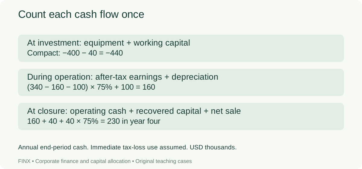
Larch Components can install one of two production lines. The Compact line costs 400 and ties up another 40 in inventory and receivables. The Automated line costs 700 and ties up 70. Both operate for four years. All amounts are USD thousands. These are original fictional assumptions, not company disclosures or current tax rules.

The relevant question is what changes if Larch accepts the project. A 20 feasibility study already paid is sunk. A 12 annual rental income forgone by using a building is an opportunity cost, even when no new invoice arrives. Include sales lost elsewhere through cannibalization. Exclude allocated head-office costs that will not change. Include incremental support staff or capacity costs even if they sit in a different department.

Separate operating investment from financing. This case discounts cash available to debt and equity investors at a project WACC. Deducting interest in those flows would count financing again. A cash flow after debt payments instead needs an equity-specific model and discount rate.

Annual operating schedule	Compact	Automated
Revenue	340.00	570.00
Cash operating cost	(160.00)	(270.00)
Straight-line depreciation	(100.00)	(175.00)
EBIT	80.00	125.00
Incremental tax at 25%	(20.00)	(31.25)
Add back depreciation	100.00	175.00
Operating cash flow	160.00	268.75

The 25% rate and straight-line tax depreciation are teaching assumptions. The parent has enough taxable profit to use incremental losses immediately. If it cannot, loss carryforwards and cash-tax timing need a different schedule. Book depreciation does not automatically determine tax deductions in practice.

At time zero, buy the line and fund working capital: −440 for Compact and −770 for Automated. Working capital remains flat during operation and is fully recovered after year four. Depreciation takes tax book value to zero. Compact sells for 40, giving after-tax proceeds of 40 − (40 − 0) × 25% = 30. Add 40 of working-capital recovery: final cash is 230. Automated final cash is 398.75: operating cash 268.75, after-tax sale 60 and recovery 70.

Check: Compact cash flows are −440, 160, 160, 160, 230. Automated flows are −770, 268.75, 268.75, 268.75, 398.75. Recover working capital once; it is not revenue or taxable operating profit in this case. With a nonzero disposal tax basis, use sale − tax × (sale − tax basis), subject to the assumed tax treatment.

Try it: A proposed line has annual sales 420, cash costs 230, forgone rent 12 and cannibalized after-variable-cost contribution 18. Depreciation is 100. Derive EBIT and operating cash at 25% tax before looking below.

Reasoned solution: incremental cash operating surplus is 160; EBIT is 60; tax is 15; operating cash is 145. The already-paid study is excluded. Do not subtract its 20 again.

Transfer question: If only 75% of the 40 working-capital balance is recovered, how much lower is the final cash flow? It falls by 10. At a 10% annual discount rate, value today falls by 10 / 1.1^4 = 6.83.

Optional reading: OpenStax capital budgeting.

2. Choose value before ranking percentages

Outcome: compare mutually exclusive projects using NPV, interpret IRR and payback, and detect nonconventional cash flows. Prerequisite: lesson 1.

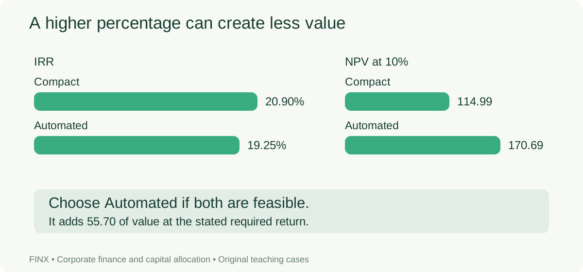
Compact earns a higher percentage return. Automated adds more value at the stated 10% required return. Before calculating, predict which line Larch should choose if both are affordable and their risk and life are comparable.

Discount each annual cash flow to time zero: PV = cash / (1 + rate)^year. Add the negative initial investment without discounting it. Excel’s ordinary NPV starts discounting its first cash-flow argument one period from now. With time zero in C5 and years 1–4 in D5:G5, use =C5+NPV(rate,D5:G5). Passing C5:G5 into NPV discounts the initial outlay too.

Four-year investment	Compact	Automated
Initial cash required	440.00	770.00
NPV at 10%	114.99	170.69
IRR	20.90%	19.25%
Simple payback, assuming even annual operating receipts	2.75 years	2.87 years

IRR is the discount rate that sets the project’s NPV to zero. Compact’s higher IRR does not tell us how much total value it creates. Automated requires 330 more and adds 55.70 of present value. Under these assumptions and with capital available, choose Automated. If the extra capital is unavailable, that feasibility constraint changes the choice.

Payback answers a timing question about recovering the initial outlay. Simple payback ignores the time value of money and cash after the cutoff. Discounted payback corrects only the first weakness. Here the fractional-year figures assume receipts arrive evenly; the formal valuation assumes end-year flows. On a strict year-end basis, both recover their undiscounted outlays at year 3. Use the convention that fits the decision and label it.

An IRR acceptance rule works cleanly for an initial outflow followed by inflows when the required return is appropriate. It can mislead for scale differences, timing differences, financing-style cash flows and nonconventional sign changes. For −100, +230, −132, both 10% and 20% are IRRs. At 15%, NPV is about +0.19. A spreadsheet’s single returned root is not a complete decision rule. Inspect the NPV profile and use the chosen required return.

Check: prove both roots by direct discounting. At 10%, −100 + 230/1.10 − 132/1.10^2 = 0; at 20% the same identity holds. Do not force an iterative IRR function to choose your preferred root.

Try it: At 10%, project A costs 100 and returns 130 in one year. B costs 500 and returns 620. Which has the higher IRR, and which creates more value if they are mutually exclusive and both feasible?

Reasoned solution: A has 30% IRR and 18.18 NPV; B has 24% IRR and 63.64 NPV. Choose B on NPV under the stated constraints. It creates 45.45 more value.

Transfer question: Would borrowing at 6% make 6% the correct project discount rate? No. Debt pricing measures one financing claim; required project returns must reflect the risk of the operating cash flows.

Optional reading: OpenStax on IRR.

3. Allocate a limited budget across feasible combinations

Outcome: choose a value-maximizing set of indivisible projects under a capital constraint. Prerequisite: lesson 2.

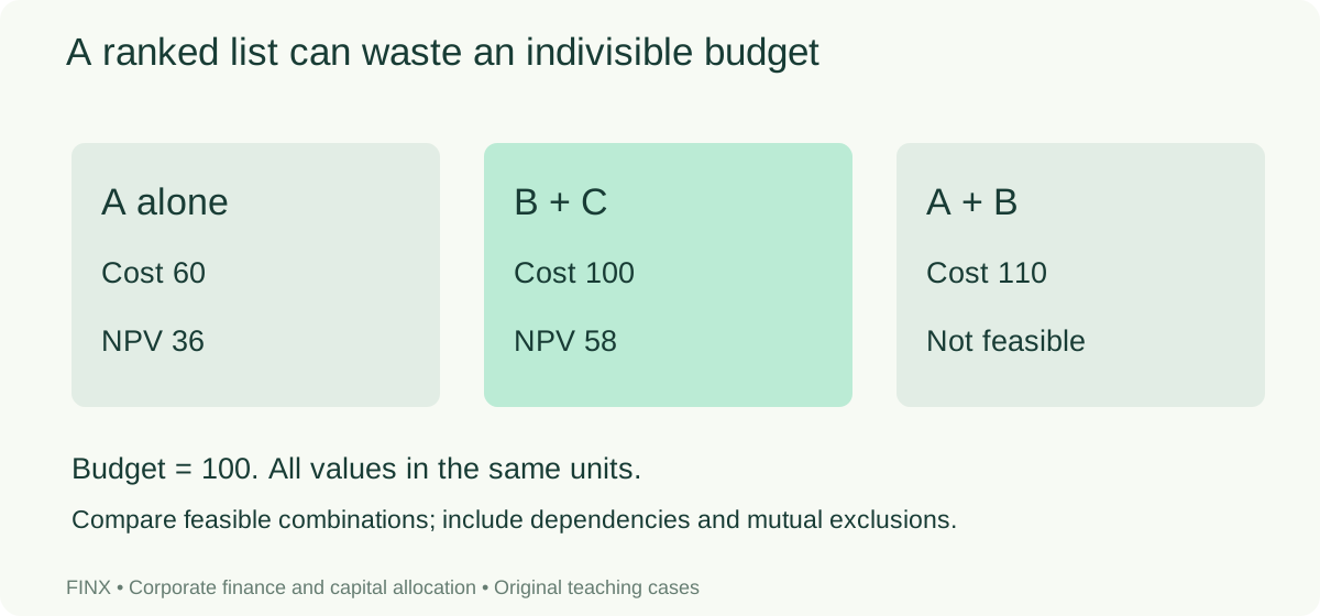
A company cannot always fund every positive-NPV project. It may face a real financing limit or an internal budget. First document the limit: time-zero cash, staffing, production capacity, a later-year funding need, or a policy that management can change. A single initial budget does not prove the company can fund later cash needs.

For independent, divisible projects under one binding cash constraint, a profitability index can help prioritize. With a single initial outlay, PI = PV of future inflows / initial investment = 1 + NPV / investment. Real projects are often indivisible and may be mutually exclusive or dependent. Ranking ratios alone can leave money stranded.

Consider three independent, indivisible projects with only time-zero budget requirements. Their supplied NPVs were calculated at consistent risk-adjusted rates.

Project	Initial investment	NPV	Profitability index
A	60	36	1.60
B	50	29	1.58
C	50	29	1.58

The budget is 100. Choosing the top ratio, A, leaves 40 that cannot buy B or C. NPV is 36. Choosing B and C uses 100 and creates 58. Enumerate feasible combinations: none, A, B, C and B+C. A+B, A+C and A+B+C exceed the limit. The right comparison is the value of feasible portfolios, including doing nothing.

For two mutually exclusive machines that provide the same repeatable service but have different useful lives, compare equivalent annual cost only if repeated replacement is credible, service levels are comparable and costs/rates have consistent treatment. This course’s existing “Machines with Different Lives” exercise covers that arithmetic. For a finite one-off decision, use an explicit common planning horizon and residual values instead of assuming replacement forever.

Check: at a budget of 110, A+B and A+C each create 65 and beat B+C. A tie needs a stated nonfinancial criterion; it does not license an arbitrary claim of superiority.

Try it: With a budget of 90, which combination above is feasible and best? A creates 36, versus 29 for B or C; no two-project combination fits. Changing the budget can change the winning set abruptly.

Transfer question: What if C works only after A is installed? B+C is no longer feasible without A. Rebuild the allowed combinations before comparing their values.

4. Match required return to the risk being priced

Outcome: distinguish diversification, systematic risk and project uncertainty, then interpret beta. Prerequisite: F01 probability and weighted averages.

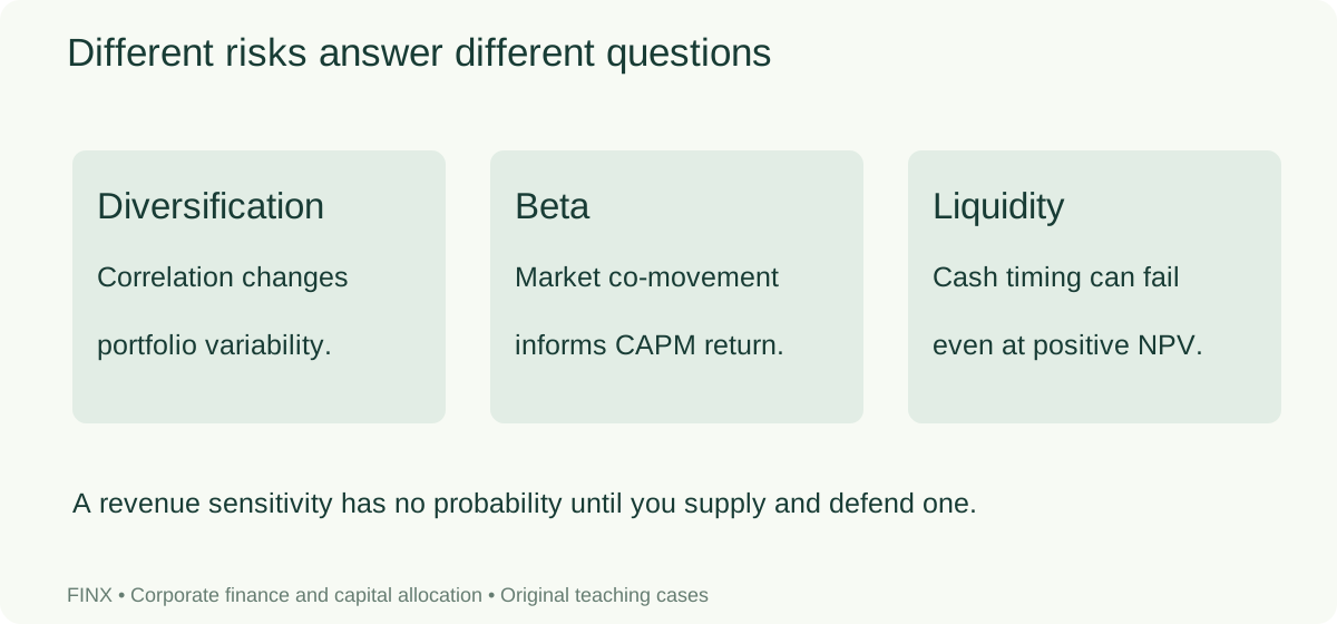
A project can have uncertain outcomes without all of that uncertainty commanding a market risk premium. In the standard diversified-investor framework, some firm-specific risks can be diversified across holdings. Economy-wide risks remain. CAPM uses beta to describe sensitivity to market returns, not total volatility or the probability of a project’s failure.

An equal-weight portfolio of two assets each with 20% volatility has 20% portfolio volatility if correlation is +1, about 14.14% if correlation is zero, and zero in the idealized perfectly offsetting −1 case. The last result is an arithmetic illustration, not a claim that a dependable real-world hedge exists. Correlations, weights and exposures can change precisely when protection matters.

For two assets, variance is wA^2 × σA^2 + wB^2 × σB^2 + 2 × wA × wB × ρ × σA × σB. Take its square root for volatility. Expected portfolio return is the weighted average of expected returns. Lower volatility alone does not guarantee higher expected return.

CAPM estimates cost of equity = risk-free rate + equity beta × market risk premium. At an assumed 4% risk-free rate, 1.4 beta and 6% premium, cost of equity is 12.4%. These are fictional teaching inputs, not current market estimates. Beta estimated from a short return sample is noisy; choice of market, frequency, period and capital structure matters.

Larch’s 10% project rate assumes the two lines have similar operating risk to the business used to estimate its cost of capital. A speculative new overseas product would need its own risk analysis. Applying one corporate hurdle to every project can favor riskier cash flows. Using a high rate as a substitute for explicitly modeling a delay or failure can also hide what actually goes wrong.

Check: increasing beta from 1.4 to 1.6 increases estimated cost of equity by 1.2 percentage points, to 13.6%, with other assumptions unchanged. It does not mean the investment is guaranteed to earn that return.

Try it: Two equally weighted assets have volatilities of 20% and 30%, with zero correlation. Portfolio variance is 0.0325 and volatility is about 18.03%. Explain why averaging 20% and 30% gives the wrong risk figure.

Transfer question: Would diversification inside a company automatically make a project valuable? No. Compare incremental cash flows and required returns; diversified shareholders may already obtain diversification themselves.

Optional reading: OpenStax CAPM.

5. Build WACC with consistent claims and conventions

Outcome: calculate a market-weighted WACC and explain when it is appropriate. Prerequisite: lesson 4 and the existing cost-of-capital exercises.

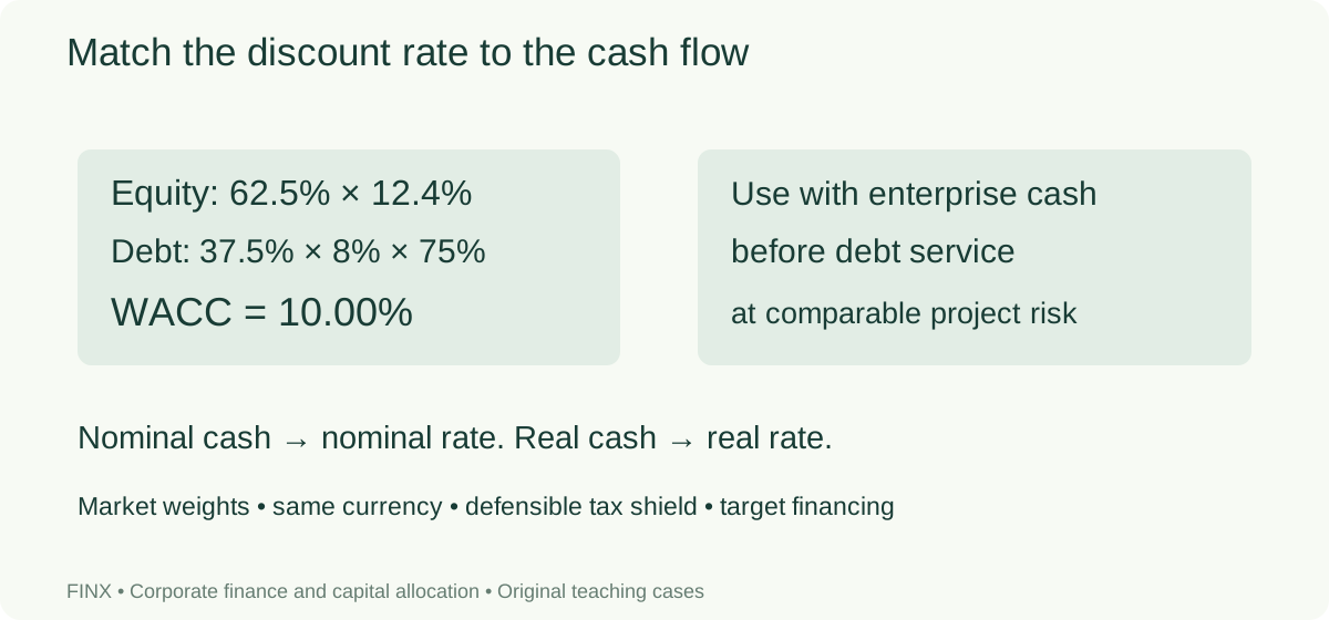
Debt and equity are different claims on the same business. The required return on equity is not a dividend yield, and the marginal cost of debt is not necessarily the coupon printed on an old bond. The existing bond exercise derives yield from the bond price and cash flows. For a new decision, use a supported current borrowing cost for comparable risk and tenor.

Teaching assumption	Value
Market equity value	1,000
Market debt value	600
Cost of equity	12.4%
Pretax cost of debt	8.0%
Marginal tax rate with usable deduction	25.0%

Equity weight is 62.5%; debt weight is 37.5%. After-tax debt cost is 6.0%. Therefore WACC = 62.5% × 12.4% + 37.5% × 8% × (1 − 25%) = 10.0%. Weights sum to 100%. Tax affects the debt term once. It does not reduce cost of equity.

Use market values or a justified target market capital structure. Accounting book equity records historical transactions and is not automatically the opportunity cost of funding. Keep the valuation date, currency, nominal/real basis, annual timing and cash-flow claim aligned. Nominal USD after-tax unlevered cash flows need a compatible nominal USD after-tax project discount rate. If nominal return is 10% and inflation is 2%, the exact corresponding real return is 1.10 / 1.02 − 1 = 7.84%.

Leverage changes equity risk. Under a simplified zero-debt-beta convention, unlevered beta = levered beta / [1 + (1 − tax) × D/E]; relever to a new target D/E before estimating equity cost. With beta 1.4, tax 25% and D/E 0.6, unlevered beta is 0.966. At target D/E 0.3, relevered beta is 1.183. This shortcut has assumptions about debt risk and tax shields; it is not a universal identity for every financing structure.

More debt does not mechanically lower WACC forever. Credit spreads, equity risk, refinancing exposure and expected distress costs can rise. If tax deductions are restricted or unusable, the simple after-tax cost overstates the shield. Changing leverage materially can call for a period-specific financing model or an adjusted-present-value approach.

Try it: Remove the usable tax shield while holding the supplied claims and required returns fixed. WACC becomes 10.75%. This isolates one assumption; it is not an equilibrium forecast after a change in tax law.

Transfer question: Why should an analyst avoid mixing real cash flows with a nominal WACC? Inflation would be removed from the cash flows but retained in the discount rate, understating their value under otherwise consistent assumptions.

Optional reading: OpenStax capital structure.

6. Separate financing feasibility from payout arithmetic

Outcome: compare debt, equity, dividends and buybacks while preserving liquidity and recognizing dilution. Prerequisites: F03, F07 for integrated application.

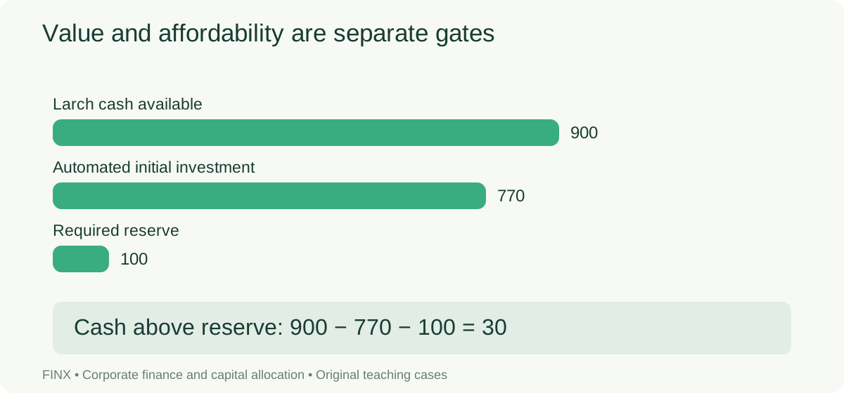
Positive NPV does not mean a company has the cash to execute. Larch has 900 at time zero and requires a 100 reserve. Automated needs 770, leaving only 30 above the reserve. A 60 distribution would create a 30 shortfall, even though the project’s NPV is positive. Later annual inflows cannot fund an initial cash payment without bridging finance.

If cash is only 650, the 770 investment and 100 reserve require 220 of new funding. A committed unused facility of 150 leaves an unfunded gap of 70. Required borrowing is a calculation; committed borrowing is an actual financing limit. Covenant compliance, monthly timing, fees, amortization and interest must be added before relying on a financing plan.

Equity avoids contractual principal repayment but dilutes ownership. Raising 200 net at a price of 20 per share with 2% issuance fees requires gross proceeds of 200 / 98% = 204.08. That is 10.204 thousand new shares. If 100 thousand shares already exist, new investors own 10.204 / 110.204 = 9.26%. Net cash raised and ownership dilution are different quantities.

A buyback can raise EPS without creating operating value. With net income 100 and 100 thousand shares, EPS is 1.00. Repurchase 10 thousand shares for 200 at 20 per share. If earnings otherwise remain 100, EPS becomes 1.11. The firm also loses 200 cash and its future interest income or investment options. Buying shares above their value can hurt continuing owners despite higher EPS. Debt-financed repurchases also change risk and interest expense.

Dividends distribute cash pro rata; repurchases change the share count and who continues to own the business. Taxes, signaling, transaction costs, investor preferences, authorization and local law can matter. This lesson supplies arithmetic and decision questions; no jurisdiction-specific tax or legal treatment is assumed.

Check: the 30 residual is a maximum under this simplified time-zero cash rule. It is not a board recommendation or proof of future liquidity. Compare retaining the cash, financing the project differently and reducing or deferring the payout.

Try it: With 120 of net income, 100 shares and a 20-share buyback, unchanged-earnings EPS rises from 1.20 to 1.50. State what the calculation leaves out before calling it value creation.

Transfer question: What if the repurchase price falls? The same cash buys more shares, but that fact alone says nothing about intrinsic value, financing risk or the best use of capital.

7. Ask what the next unit of capital earns

Outcome: connect operating returns, reinvestment and growth without treating growth or EPS as value by themselves. Prerequisite: F05 return-on-capital analysis.

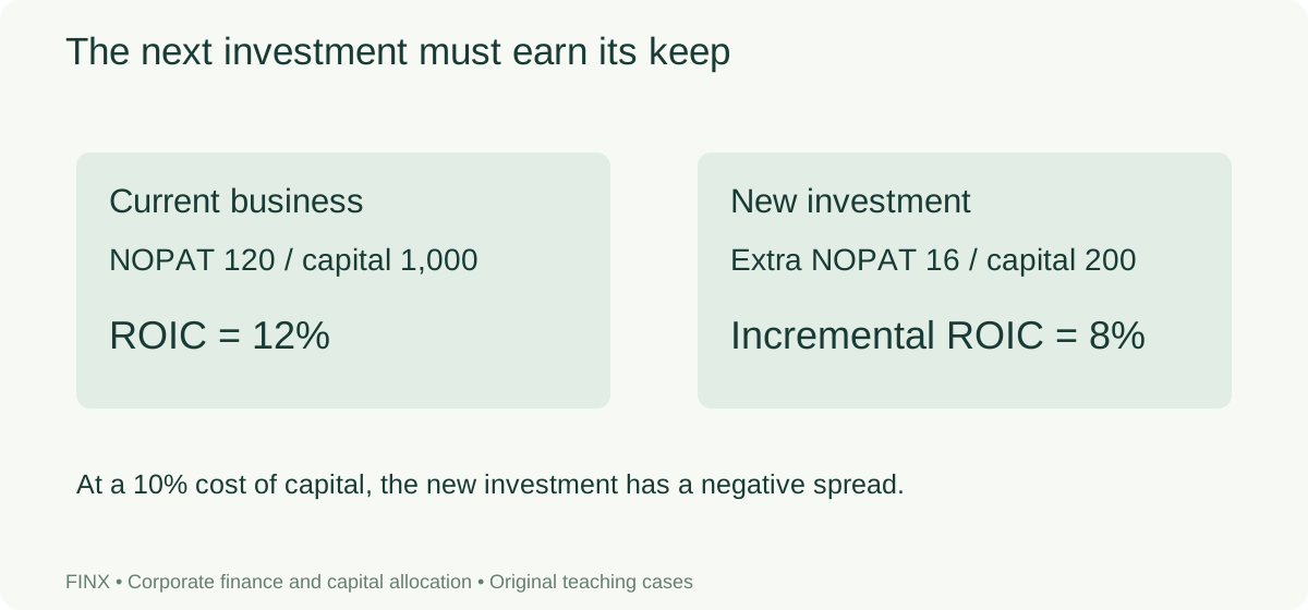
Return on invested capital compares after-tax operating profit with the capital employed to earn it. For this example, NOPAT is 120 and opening operating invested capital is 1,000. ROIC is 12%. At a 10% cost of capital, the annual economic-profit illustration is 120 − 10% × 1,000 = 20. Keep the denominator convention explicit; opening versus average capital, acquisitions, impairments, leases and expensed intangibles can change the reported ratio.

The next project may not earn the historical average. If another 200 of investment produces 16 of incremental annual NOPAT, its incremental ROIC is 8%, below the assumed 10% required return. The annual capital-charge illustration is −4. That warning does not replace a complete dated NPV, including the initial outlay, duration, reinvestment and terminal cash flows.

Under stable operating-return and reinvestment assumptions, growth in operating earnings can be approximated by reinvestment rate × return on new capital. Reinvesting 50% at 12% produces 6% growth; reinvesting the same proportion at 8% produces 4%. Faster growth at sub-hurdle returns can consume value. Better returns on existing capital can also produce earnings growth without the same new-investment relation.

Business unit	Incremental investment	Annual incremental NOPAT	Incremental ROIC	Annual profit less 10% capital charge
Parts	200	30	15%	10
Service	200	16	8%	(4)

Do not blindly allocate everything to the 15% unit. Ask how much can be invested at that return, how long it lasts, whether the risks differ, whether units share customers, and whether the estimates omit required support investment. The relevant comparison is the next feasible opportunity at an appropriate rate.

Try it: NOPAT is 90, net capital expenditure is 24 and working capital increases by 12. Reinvestment is 36, reinvestment rate is 40%, and unlevered free cash is 54. At a sustainable 15% return on new capital, the simplified implied growth is 6%.

Check: calculate reinvestment after depreciation when using NOPAT. Deducting gross capex without adding depreciation back mixes cash and accounting definitions.

Transfer question: Can a buyback improve ROIC by reducing operating invested capital? Buying back equity does not itself remove operating assets. Define operating capital consistently instead of letting a financing transaction manufacture operating improvement.

Optional reading: Damodaran on the determinants of growth.

8. Find the assumption that reverses the decision

Outcome: recommend an investment, diagnose an IRR trap and quantify a decision threshold. Prerequisites: lessons 1–7; F07 for a complete financing forecast.

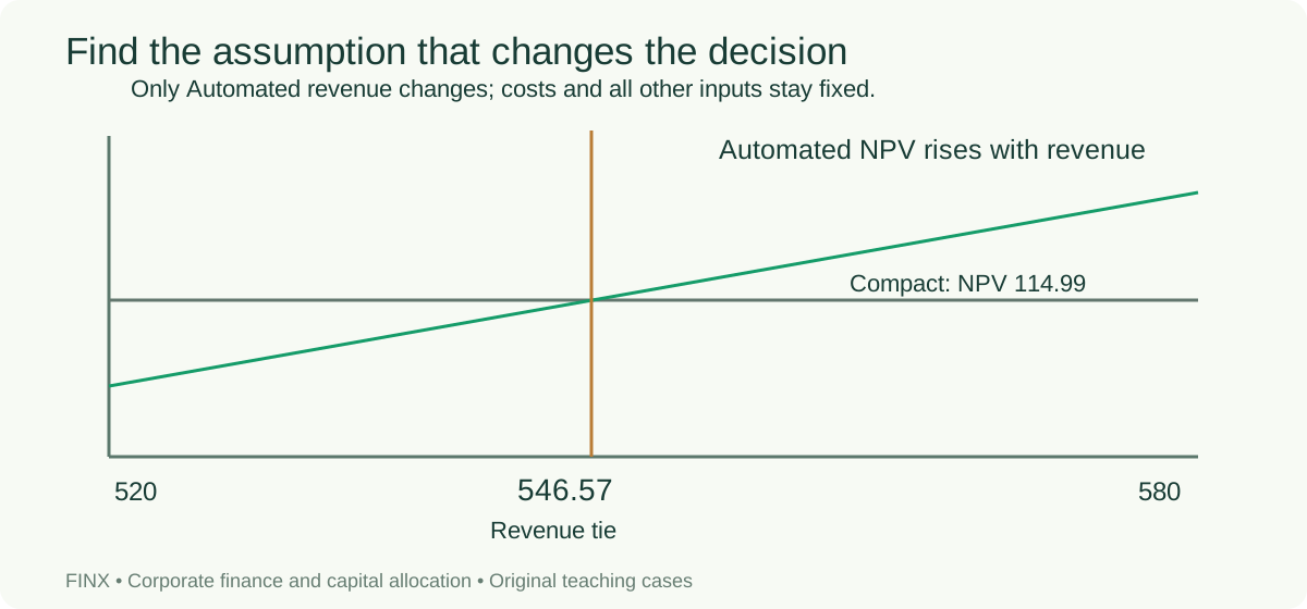
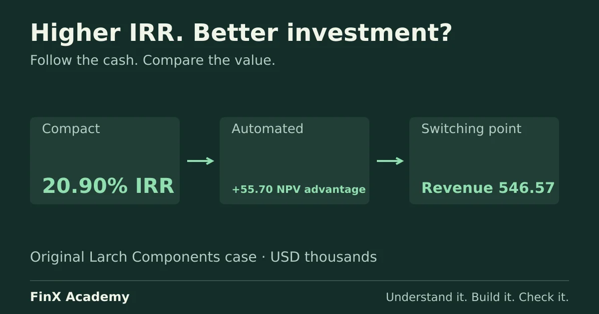
Return to Larch. Automated creates 170.69 of NPV, versus Compact’s 114.99. Its higher initial cost still fits the 800 investment capacity after the cash reserve. Compact’s 20.90% IRR exceeds Automated’s 19.25%, but Automated adds 55.70 more value at 10%. The recommendation is conditional on those cash, risk and timing assumptions.

Hold Compact and all other Automated inputs fixed. Each 1 of Automated annual revenue changes after-tax operating cash by 0.75 in each of four years. The four-year annuity factor at 10% is 3.169865. Each 1 of revenue therefore changes NPV by 2.377399. Divide the 55.703675 NPV advantage by 2.377399: Automated can lose 23.43049 of annual revenue before the projects tie. The switching revenue is 546.57, about 4.11% below 570.

This is a relative choice threshold, not Automated’s zero-NPV revenue. Below 546.57, Compact can become preferable even while Automated remains positive-NPV. At revenue 540, Automated NPV is 99.37 and Compact wins by 15.62. If revenue falls, costs or working capital may change too; a one-variable sensitivity deliberately holds those fixed. A scenario changes a coherent set of assumptions. Neither provides a probability by itself.

Try it before revealing the model: change Automated revenue to 540, then increase time-zero capex by 50. Recalculate depreciation, taxes, initial cash, NPV and remaining liquidity. Do not change only the displayed NPV. Record the input, affected formulas and recommendation, then restore the original case.

For probability-weighted scenarios, state the probabilities and ensure they sum to one. Expected NPV is the weighted mean of conditional NPVs when the modeling convention is consistent. It is not the NPV guaranteed to occur and says nothing by itself about the chance of a cash shortfall. Do not count the same conservatism both in cash flows and a discount-rate premium without explanation.

Unfamiliar transfer: Cedar Packaging

Use the separate blank Cedar workbook. Cedar can install only one of the following lines, both for four years. Tax is 30%, required return 12%, cash 760 and the time-zero reserve 80. Tax depreciation is straight-line to zero. All operating cash arrives at year end; working capital is funded at time zero, held constant and fully recovered in year four. Sale proceeds are taxed against zero basis; incremental losses can be used immediately by the parent.

Input, USD thousands	Refit	Replace
Capex	300	600
Initial working capital	30	60
Annual revenue	280	500
Annual cash cost	140	250
Year-four sale proceeds before tax	30	60

Build the dated cash flows, NPVs, IRRs and cash after investment. Recommend a feasible choice. Find Replace’s annual revenue at which the two NPVs tie, verify the threshold by recalculation, and test one revenue value on each side. Identify the IRR ranking trap. Then reduce cash to 700 and explain what happens to the feasible set before assuming new finance.

Submission and self-review rubric

Submit the workbook, a changed-input test log and a 150–250 word allocation memo. Include the decision, quantified NPV advantage, funding condition, IRR limitation, switching assumption, evidence still needed and one next action. Numerical grading checks specified formulas and values. The business recommendation, probabilities, risk assumptions and written reasoning require self-review or an identified reviewer.

Use the separate solution only after an independent attempt. This public learning assessment is not a secure hiring test. A complete submission: (1) includes all incremental flows once; (2) uses consistent claims, tax, timing and discount rates; (3) compares feasible choices including neither; (4) responds correctly to changed inputs; and (5) states a conditional, evidence-based recommendation. Review each unmet item explicitly rather than assigning an invented automated memo score.

Continue in the spreadsheet

Start the four free F08 exercises. Build cash flows and diagnose ranking traps, then continue with full access for constrained allocation, risk, financing and the unfamiliar decision case.