Integrated three-statement modelling: can the plan fund itself?

Ridgeway Pumps reports a profit, but its growth ties cash up in invoices and inventory. Can it fund its operating plan while keeping at least 75 of annual closing cash, within a 150 committed revolver? Build the model and find out. This is an original fictional teaching case, with money in USD thousands.

Prerequisites: F03 accounting, F04 source reconciliation, F05 financial statement analysis, and F06 model architecture. This extension reuses The 3-Statement Build; the original twenty cumulative exercises and your progress remain. F07 adds eight written lessons and sixteen native exercises. Four of the new exercises are free, alongside the original two free exercises. Full access continues into supporting schedules, funding and the unfamiliar native case. The written lessons and downloads below are public practice materials.

Download the Ridgeway starter and the substantially blank Atlas assessment. Attempt them before opening the separate Ridgeway solution or Atlas solution. The source pack includes historical statements, assumptions, source notes, answer references and the handoff template. This is a learning assessment; the public solutions make it unsuitable as a secure hiring test.

The final submission is a working five-year model, a scenario/input/error test log, and a 150–250 word funding recommendation. Formula grading checks calculations. Accounting choices, driver credibility, funding availability and the written handoff require analyst review.

1. Reconcile history before forecasting

Outcome: prove the opening statements reconcile and defend an operating driver. Prerequisite: F03–F06.

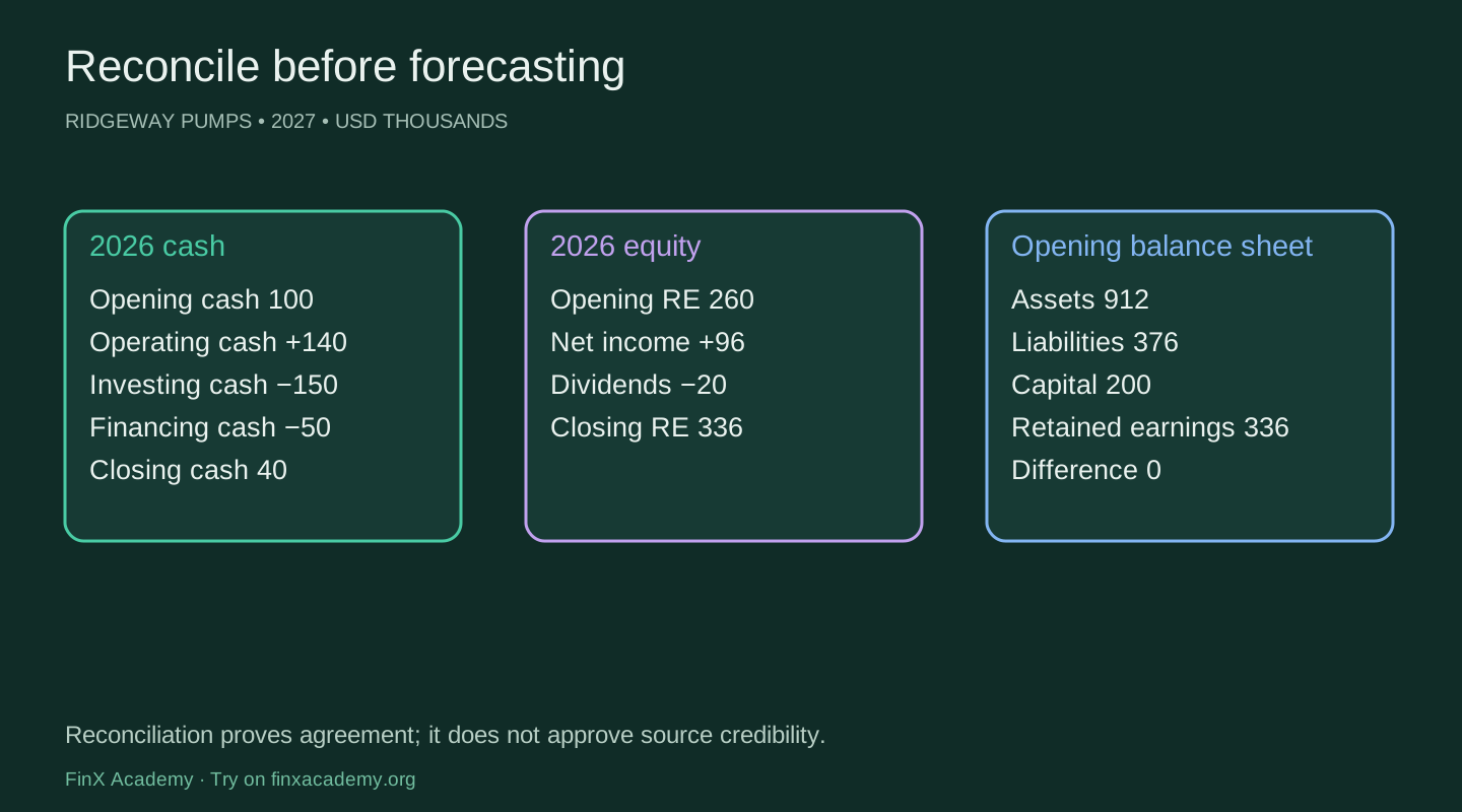
Ridgeway Pumps earns 96 in 2026 and ends with just 40 of cash. Management wants to grow, spend 132 on equipment and software, repay its lender and keep at least 75 in cash. Can the plan fund itself? All monetary figures are USD thousands. Volume is thousands of pumps; price is USD per pump. The business and source pack are original fictional teaching data.

Start with the supplied 2024 opening balances and the 2025–2026 statements. Do not estimate retained earnings to make a forecast balance. In 2026, assets of 912 equal operating liabilities and debt of 376 plus equity of 536. Retained earnings independently roll from 260 to 336: 260 + 96 profit − 20 dividends. Cash rolls from 100 to 40: 100 + 140 operating cash − 150 investing cash − 50 financing cash. If those controls disagree, investigate source periods, signs, missing accounts and transactions before adding forecasts.

Historical driver	2025	2026	What it can support
Volume, thousand pumps	10	12	20% historical volume growth
Price, USD/pump	100	100	No observed price growth
COGS / revenue	60%	60%	A base starting point, not a guaranteed margin
Receivables / revenue	14%	15%	Collection timing deserves investigation
Inventory / COGS	20%	20.83%	Closing inventory increased faster than sales

The base forecast assumes 15% volume growth and 3% pricing in 2027. Those are management assumptions, not historical facts. Defend them with order backlog, capacity, customer renewal and pricing evidence. Two observations cannot establish a reliable trend or prove that higher prices will not reduce volume. Use the downside to expose the consequence of being wrong.

F06 supplied the architecture. Here, Assumptions feeds Operations, Working capital, Assets and Funding. Statements reads their results. Review observes reconciliations and never funds the business or changes another schedule. Historical inputs stay separate from scenario inputs. Forecasting begins from the reconciled 2026 close, not an invented opening balance.

Practice: reconcile 2026 retained earnings and cash, then calculate revenue growth as volume and price effects. State one additional source needed to defend next year’s volume assumption.

Hint 1: cash is a stock and CFO is a period flow. Hint 2: include capex, principal and dividends. Checkpoint: revenue grew 20%; cash fell 60; retained earnings grew 76.

Review judgment: numerical checks prove the supplied records reconcile. They cannot prove the source pack is complete or that management’s assumptions are credible.

2. Build revenue and operating costs

Outcome: forecast units, price, margins and cash operating expenses through one set of selected assumptions. Prerequisite: lesson 1.

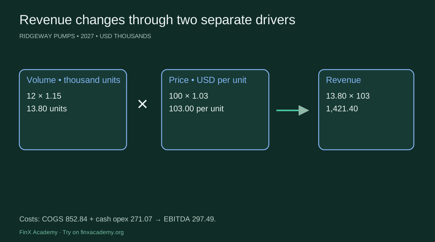
Before changing the workbook, predict whether 15% more pumps and 3% higher prices produce 18% revenue growth. The exact answer includes the interaction: 1.15 × 1.03 − 1 = 18.45%. A price-volume build exposes this mechanism.

Volume rolls from 12 to 13.8 thousand pumps. Price rolls from 100 to 103 dollars. Revenue is 13.8 × 103 = 1,421.40 in USD thousands. Do not divide by a thousand again: the volume already uses thousands. COGS at 60% is 852.84, leaving gross profit of 568.56. Fixed cash opex of 200 plus variable opex of 5% of revenue gives 271.07. EBITDA is 297.49.

Step	Formula meaning	2027 base
Volume	Prior volume × (1 + volume growth)	13.80
Price	Prior price × (1 + price growth)	103.00
Revenue	Volume × price	1,421.40
Cash opex	Fixed opex + revenue × variable share	271.07
EBITDA	Revenue − COGS − cash opex	297.49

Margin and expense drivers describe different economics. A COGS share is a simplification for materials and conversion cost. Fixed opex has its own budget; it should not automatically scale with revenue. Depreciation and amortization are outside this cash-opex input and join the income statement from Assets. Keeping them separate prevents a double charge.

The selected scenario supplies every period’s active assumptions. Change the selector once and watch the same formulas recalculate. Change only the 2027 price-growth input from 3% to 4% for a sensitivity, then restore it. Revenue becomes 1,435.20, a rise of 13.80; with unchanged cost shares EBITDA rises 4.83. Later years compound from the changed price, so the effect continues.

A realistic forecast also needs capacity, demand, product mix, seasonality and cost inflation evidence. This annual single-product case assumes capacity is sufficient and all recognized sales are collectable. Those assumptions require review. Do not interpret the model’s five-year horizon as a five-year forecast confidence interval.

Practice: build the first year, fill across, switch to Downside and restore Base. Explain why a price increase changes more than revenue.

Hints: link the active driver, keep growth rates as percentages, and test the next year’s opening volume. Checkpoint: EBITDA 297.49 precedes the asset, interest and tax charges.

3. Follow an invoice into cash

Outcome: link receivables, inventory, payables, prepaids and accruals to operating cash. Prerequisite: lesson 2.

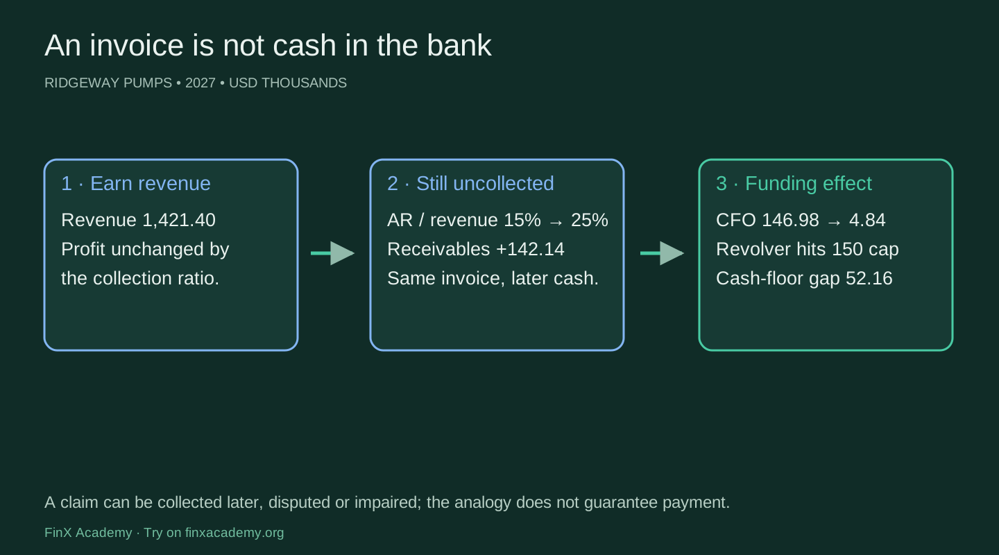
Follow one invoice. On sale, revenue is recognized and the unpaid amount becomes a receivable. Collection changes receivables into cash without creating a second sale. In aggregate, cash collected equals revenue + opening receivables − closing receivables, assuming no write-offs, acquisitions, FX or other reconciling items.

In 2027, receivables at 15% of 1,421.40 are 213.21. Opening receivables are 180, so the increase of 33.21 consumes cash. Inventory at 25% of COGS becomes 213.21, consuming another 63.21. Payables at 15% of COGS become 127.926, providing 19.926 of cash relative to paying every supplier immediately.

Prepaids equal 10% of cash opex, or 27.107, an increase of 3.107. Accruals also equal 27.107, but decline from 36; paying that prior obligation consumes 8.893. The combined operating working-capital cash adjustment is −88.494. The same closing balance does not imply the same cash effect: the opening balance matters.

Increase in a balance	Cash adjustment
Receivables, inventory, prepaids	Subtract the increase
Payables and operating accruals	Add the increase
Debt or share capital	Financing, outside operating working capital
Tax payable	Separate tax schedule in this model

Prediction: change only 2027 receivables/revenue from 15% to 25%. Profit does not change in that year under our no-bad-debt assumption. Receivables increase by another 142.14. CFO falls from 146.979125 to 4.839125. Required new borrowing rises by 142.14, but the 150 facility limit prevents a complete cash-floor restoration. The funding schedule must expose the shortage. Restore 15% after the test.

Ratios can be expressed in days: year-end DSO = receivables / annual revenue × 365. This is a closing-balance convention, not an average-balance operating metric. The base 15% is 54.75 days. Inventory and payable days use COGS as a purchases proxy. If purchases differ materially from COGS, model actual purchasing and payment terms instead. Annual snapshots can conceal monthly peaks.

Practice: construct all five balances and their signed changes, then independently calculate customer receipts, supplier payments and cash opex paid.

Hints: an asset increase absorbs cash; a liability decrease also absorbs cash. Review judgment: passing the cash bridge does not prove that receivables are collectable or that suppliers will accept those terms.

4. Roll assets forward and charge them once

Outcome: link cash capex, gross assets, accumulated depreciation and selected intangibles. Prerequisite: lesson 3.

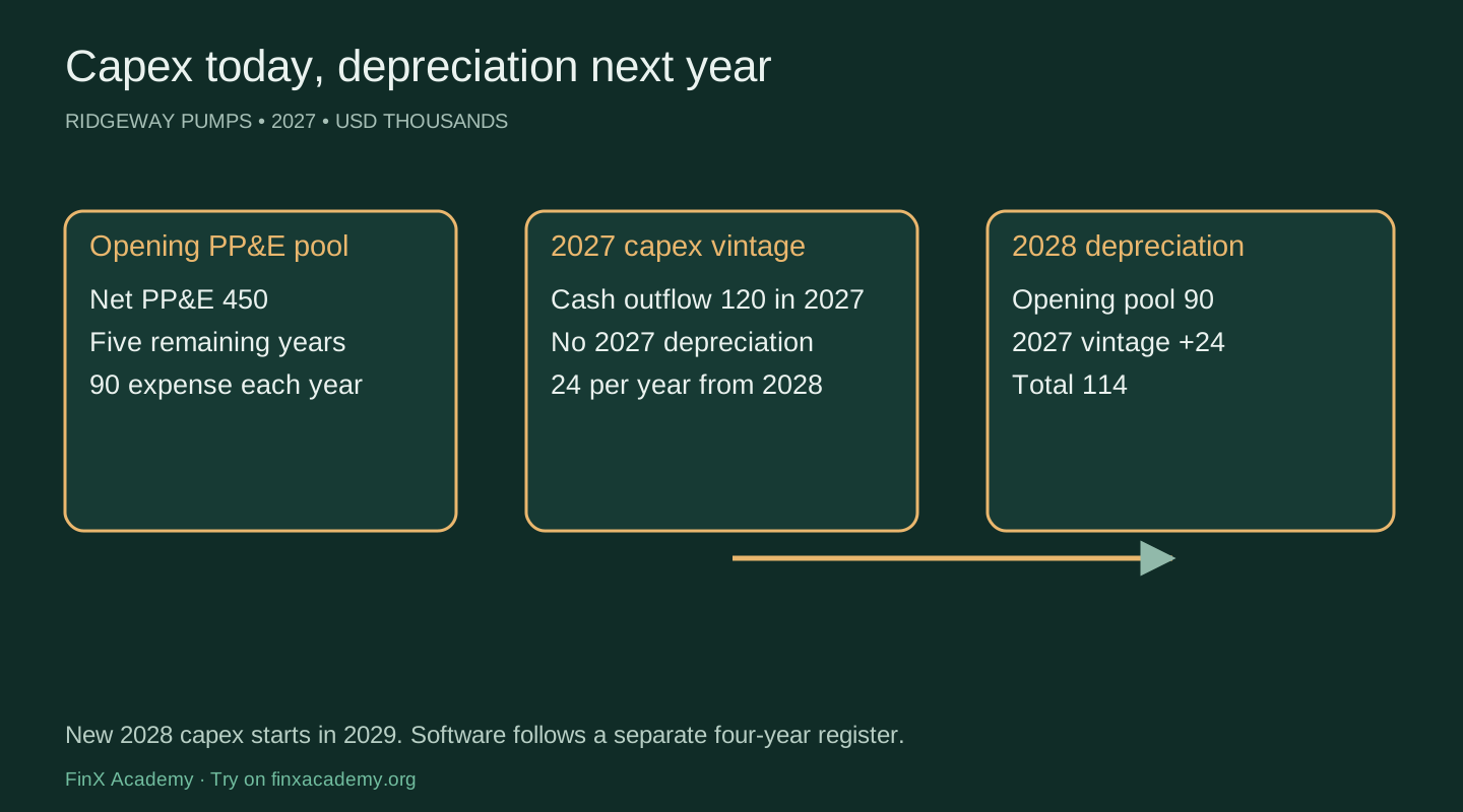
The 2026 closing PP&E balance is 450: gross cost of 880 less accumulated depreciation of 430. The supplied asset register gives the remaining 450 a five-year remaining life and no residual value. Annual depreciation on that opening pool is 90 until exhausted. This is a case fact, not a rule that net PP&E divided by an assumed life always produces the correct charge.

New capex is paid and made available for use at the final instant of each year. The teaching model therefore charges its first full year of depreciation in the next period. New vintages use five years, straight line, no residual. Year-one capex of 120 has no 2027 charge but contributes 24 in 2028. Depreciation is 90 in 2027, 114 in 2028 and 132 in 2029. A real in-service date requires the appropriate partial-period calculation.

In 2027, gross PP&E is 880 + 120 = 1,000; accumulated depreciation is 430 + 90 = 520; net PP&E is 480. The cash-flow statement records −120 in investing cash. The income statement subtracts 90 depreciation. The indirect cash-flow statement adds back the same 90, because the asset purchase was already classified as investing cash.

Purchased finite-life software follows a separate schedule. Opening net software of 68 has four years remaining, giving 17 of annual amortization. Year-end purchases of 12 begin amortizing next year over four years. Gross software becomes 127, accumulated amortization 64 and net software 63. Do not amortize goodwill as if it were this software or capitalize every operating software expense. Recognition, impairment and useful-life judgments require evidence.

The IAS 16 material and IAS 38 material explain the underlying asset principles. The case uses explicit simplified timing; it is not a statutory reporting template.

Practice: build opening balance + additions − charge = closing balance, then fill the vintage schedule through 2031. Change 2027 capex from 120 to 180 and predict both years: current-year profit is unchanged, current-year cash need rises 60, and next year’s depreciation rises 12.

Error lab: remove the depreciation link into EBIT. The income-statement charge check must fail even if another link accidentally offsets the balance-sheet difference. Repair the link and confirm both the charge and balance checks return to zero.

Review judgment: arithmetic cannot establish an appropriate useful life, capitalization policy or recoverable value. The model excludes disposals, impairment, leases, revaluation and FX; add explicit schedules if the scope changes.

5. Make the funding limit visible

Outcome: model interest, mandatory principal, capped draws, revolver repayments and term-loan cash sweep. Prerequisite: lesson 4.

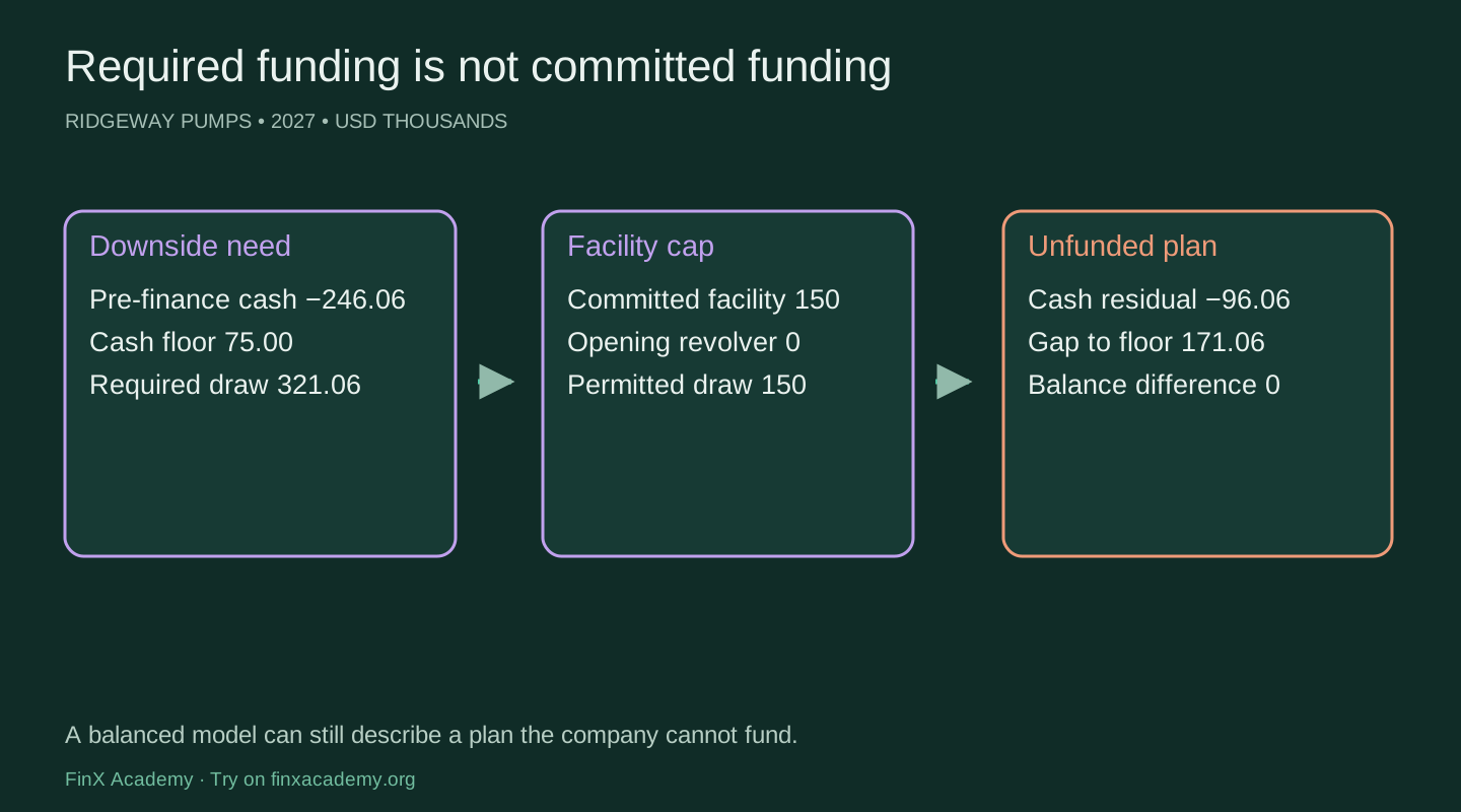
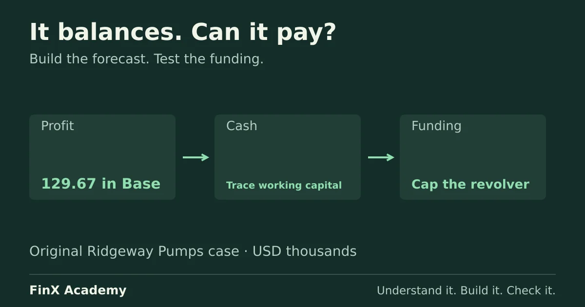
Base 2027 profit is 129.6675, but the financing decision depends on cash. Opening cash of 40 plus CFO of 146.979125 less PP&E/software spending of 132, mandatory principal of 30 and proposed dividends of 10 leaves 14.979125 before flexible financing. Maintaining 75 needs a draw of 60.020875.

The fictional facility permits 150 outstanding. Available capacity equals facility limit − opening revolver, floored at zero. Draw the smaller of the cash-floor need and available capacity. Do not set cash to 75 and make debt a balancing residual without checking the contract.

If cash before flexible financing exceeds the floor, first repay the opening revolver up to the excess. Then sweep 50% of the remaining excess into the term loan, capped at term principal after mandatory repayment. The ordering matters: do not repay the term lender while ignoring the revolver priority in this case.

Formula	Meaning
Required draw = MAX(0, floor − cash before financing)	Economic cash need
Draw = MIN(required draw, available capacity)	Permitted borrowing
Revolver repayment = MIN(opening revolver, MAX(0, cash before financing − floor))	Repay only outstanding principal
Term sweep = MIN(term after mandatory, 50% × remaining excess)	Apply the stated sweep
Closing cash = cash before financing + draw − repayments − sweep	Result, never a plug

Base 2028 cash before flexible financing is 178.71395425. Repay 60.020875 of revolver, then sweep 21.846539625 of term debt. Cash ends at 96.846539625. These movements enter financing cash and debt roll-forwards with matching signs.

Interest is 8% of opening term debt plus opening revolver. All principal movements occur at year end. Interest therefore precedes this year’s cash allocation: 17.60 in 2027, then 20.00167 in 2028. A higher current draw raises next year’s interest. Iteration is off; this is an explicit timing approximation, not a solution to an average-debt contract.

Average-debt interest plus a cash sweep can create a loop: interest → profit/tax → cash → debt → interest. The existing Alderbrook course teaches that circularity. An iterative design needs a documented loop, starting values, maximum iterations, tolerance, stress/convergence and save/reopen checks. Never silently enable iteration to hide a broken reference.

Practice: run Downside. First-year need is 321.0625, permitted draw is 150 and cash is −96.0625. The 171.0625 gap to the 75 floor is unfunded. Negative modeled cash is a diagnostic residual, not a bank balance the company can hold without additional financing. Later downside periods assume operations continue for diagnostic purposes; they are not a feasible funded plan.

Review judgment: facility availability, covenants, borrowing base, fees, daily liquidity and dividend permission need review. The simplified case assumes contractual availability up to the cap and no additional restrictions. A cash-floor formula does not establish a lending commitment.

6. Link tax, equity and the cash-flow statement

Outcome: distinguish tax expense from cash paid and link profit, dividends and equity issuance. Prerequisite: lesson 5.

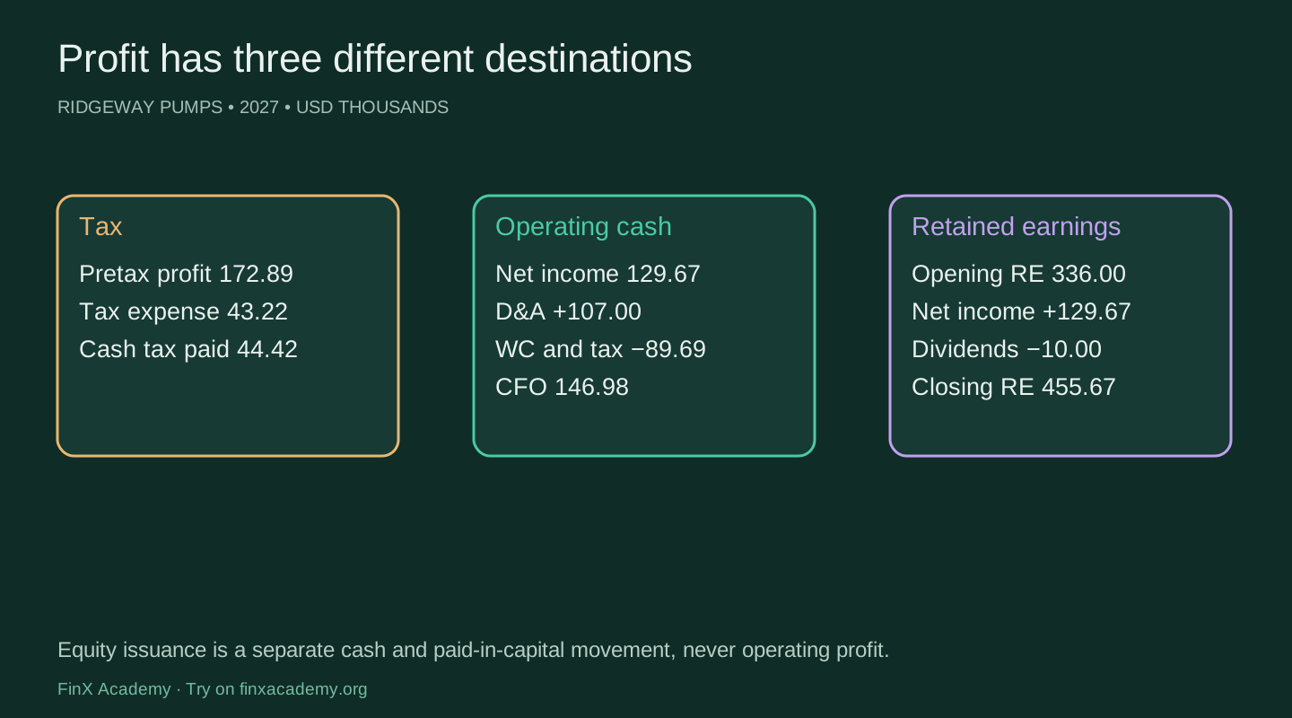
Base 2027 EBITDA of 297.49 less 90 depreciation, 17 amortization and 17.60 interest gives pretax profit of 172.89. The case charges 25% of positive pretax profit, or 43.2225. Losses produce no current tax benefit. There are no loss carryforwards, deferred taxes, permanent differences or jurisdiction-specific rules.

One quarter of the current tax expense remains payable at year end. Closing tax payable is 10.805625. Cash tax is expense + opening payable − closing payable: 43.2225 + 12 − 10.805625 = 44.416875. Cash tax exceeds expense because more prior tax is paid than new tax is deferred. Never subtract cash tax from net income a second time in the indirect bridge.

Net income of 129.6675 plus D&A of 107, the working-capital adjustment of −88.494, and the tax-payable decrease of −1.194375 gives CFO of 146.979125. Independently derive receipts and payments from the operating balances; the direct and indirect approaches must agree.

The case classifies paid interest and income tax in operating cash, equipment/software purchases in investing cash, and principal, dividends and share issuance in financing cash. This is a simplified management-model convention, not a statement that every accounting framework permits identical presentation. Reclassification changes category totals, not total cash. Check the applicable rules and effective date before statutory use; IAS 7 implementation materials are one starting point.

Retained earnings roll from 336 to 455.6675: opening RE + net income − dividends. Paid-in capital stays 200 unless the explicit equity-issuance input changes. Issuing 40 of equity supplies a 40 cash inflow and increases paid-in capital by 40; it does not create revenue or retained earnings. In this first-year base case, the funding policy reduces the revolver draw by 40, so closing cash remains at 75. Proposed equity is not automatically committed funding.

Cash-flow ending cash must tie to the financing schedule and balance sheet. In 2027, 40 + 146.979125 − 132 + 20.020875 = 75. Financing cash includes a 60.020875 draw, 30 principal repayment and 10 dividends. Never substitute a balance-sheet residual for the cash-flow result.

Practice: compute cash tax, retained earnings and the three cash categories. Increase the explicit 2027 equity input by 40 and trace the lower debt draw; restore zero. Compare this with cancelling 10 of dividends: both help liquidity, but their equity effects differ.

Error lab: replace ending retained earnings with opening RE + net income, omitting dividends. The independent RE check and balance check must detect the 10 error. Repair the roll-forward.

Review judgment: a numerical check cannot choose a tax policy, approve a dividend or confirm an equity commitment. State these unresolved decisions in the funding recommendation.

7. Integrate and diagnose

Outcome: explain statement links and localize errors without a balancing plug. Prerequisite: lesson 6.

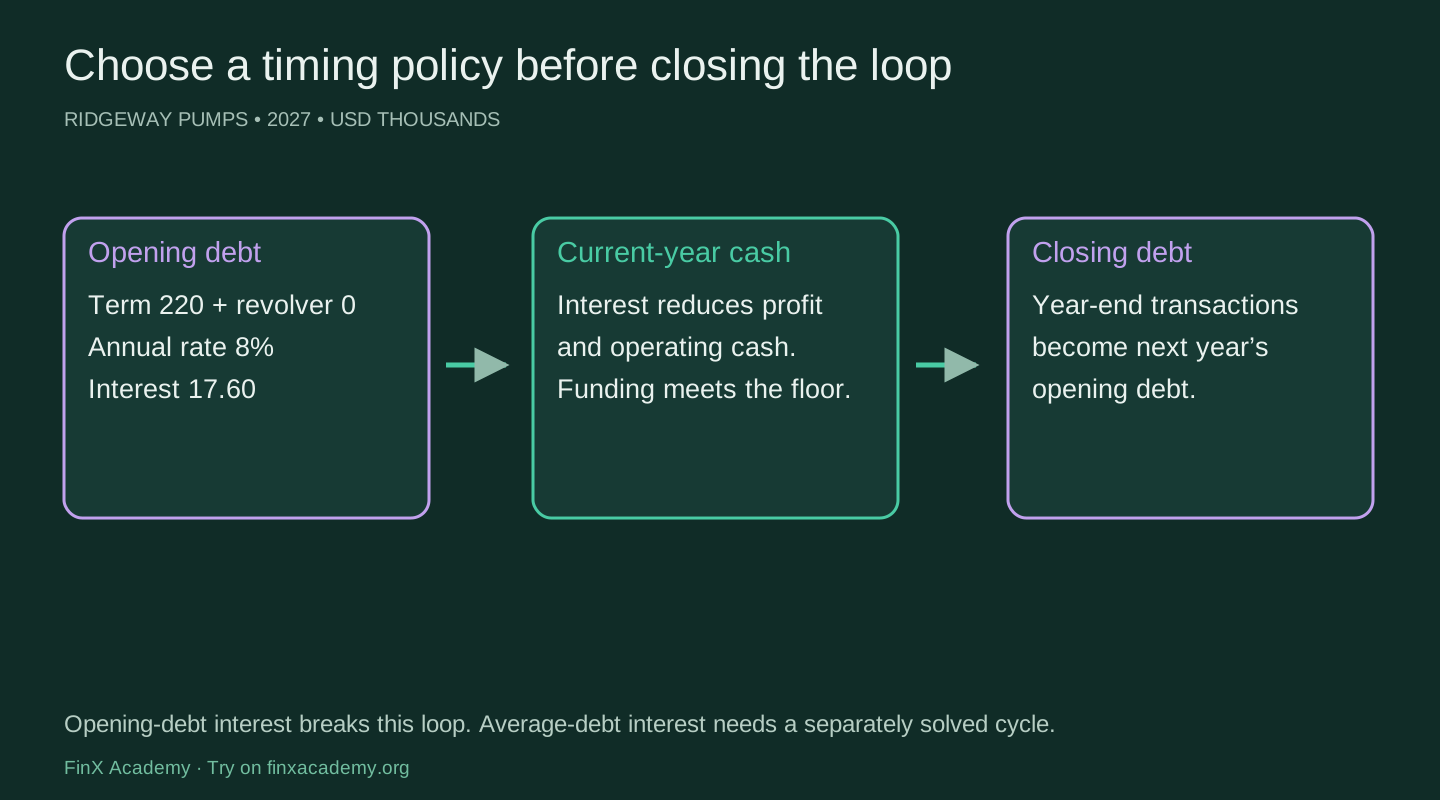
Three connections hold the integrated model together. Net income enters retained earnings and starts indirect operating cash. Closing cash from the cash-flow statement enters the balance sheet. Asset and debt schedules supply both balance-sheet stocks and the movements classified in cash flow. Revenue alone cannot connect the statements.

Use independent controls. Assets minus liabilities minus equity must be zero. Cash-flow ending cash must equal the cash-allocation schedule. Debt must equal opening debt + draws − mandatory repayment − revolver repayment − sweep. Net assets must equal gross cost minus accumulated charges, and their roll-forward must include additions and charges. Retained earnings must equal opening RE + profit − dividends. The facility headroom and cash floor are separate feasibility checks.

A balanced spreadsheet can still contain an accounting mistake. If depreciation is omitted from both expense and the cash-flow add-back, cash may remain unchanged while profit and retained earnings are overstated. Therefore compare the income-statement D&A charge with the independent asset schedule, not only the balance-sheet total.

Deliberate error	Expected detection	Repair
Reverse the receivables cash sign	Direct/indirect CFO and balance differences	Subtract closing minus opening AR
Omit the depreciation link	D&A charge check; affected earnings/equity	Link the asset-schedule charge
Omit dividends from retained earnings	RE roll-forward and balance checks	Subtract the dividend once
Draw the full need without capacity cap	Revolver capacity/policy check	MIN(need, undrawn capacity)

Run each fault separately in a copy. Record the changed formula, affected checks and numerical differences. Repair it, verify zero reconciliation differences, then start the next fault. Do not leave multiple errors offsetting one another and call the net zero a pass.

Formula consistency needs a perturbation test. A hardcoded correct base result can pass a balance check. Change an input in a later period and verify the linked revenue, tax, cash and debt change. Fill patterns must preserve fixed policy cells while moving each year’s assumptions. Compare the first, middle and final forecast columns.

Numerical comparisons use a tolerance of 0.000001 in the cell’s units. For a USD-thousands amount, that is USD 0.001. This technical floating-point tolerance is not an accounting materiality threshold. Calculations retain full precision; display rounding never becomes a hardcoded input. Blank learner cells must remain visibly incomplete rather than becoming a healthy zero. Error or missing statuses are failures to complete, not evidence of insolvency.

Practice: trace a mismatch upstream, repair all four planted errors one at a time, and restore Base. Explain which checks would fail if interest were classified in the wrong cash category but total cash still reconciled.

Review judgment: automated checks cover the listed numerical relationships. Accounting recognition, reasonable forecasts, source completeness and contractual financing interpretation still require review.

8. Decide whether the plan can be funded

Outcome: build an unfamiliar integrated forecast and deliver a short funding recommendation with a usable handoff. Prerequisite: lessons 1–7.

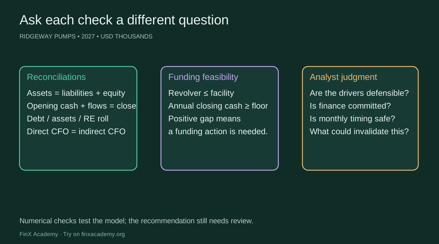
Work in three stages. First finish the labelled missing formulas in the Ridgeway starter. Then use the substantially blank Atlas Filtration assessment to build the schedules from supplied opening statements and drivers. Keep the checked solutions separate until you have attempted the work. Both cases use USD thousands, thousand units and USD per unit.

The Ridgeway base case requires a 60.020875 revolver draw in 2027 and maintains the 75 annual closing-cash floor over the first three years. Downside exhausts the 150 facility immediately, leaves a first-year cash-floor gap of 171.0625, and reaches a three-year gap of 240.974. A zero balance-sheet difference does not make that downside fundable.

Required model tests

1. Run Base, Downside and Upside in the same build. Record ending cash, peak revolver and maximum cash-floor gap.
2. Change only 2027 receivables/revenue from 15% to 25%. Explain why current-year earnings do not change while cash and borrowing do, and why next-year interest changes. Restore the input.
3. Increase year-one capex by 60. Explain the current-year cash effect and the next-year depreciation effect. Restore it.
4. Extend the horizon from three to five years. Fill the schedules and asset vintages, review the final-period references and recheck every reconciliation. The horizon does not liquidate assets or pay all debt automatically.
5. Inject and repair all four errors from lesson 7. Record failed checks and repaired outputs.
6. Complete Atlas from the labelled blank build cells. Its opening revolver is 20, facility 110, cash floor 60, term rate 9%, PP&E life four years and software life three years. Do not carry Ridgeway’s policy hardcodes into this business.

For Atlas, 2027 base revenue is 1,142.40, CFO is 120.792 and closing cash is 60 after an 11.792 revolver repayment. Those checkpoints test construction; they are not a complete answer to the business question. Switch scenarios, change a later-year operating input and extend to five years before using the separate solution.

Funding recommendation

Write 150–250 words answering whether management can fund the plan while maintaining minimum cash. State the scenario and horizon, required draw, capacity and remaining gap. Recommend a concrete next action: validate collections, defer discretionary capex, suspend proposed dividends or secure additional committed capital. Quantify the modeled effect of one action, identify its business tradeoff and avoid treating a suggested financing source as already received.

An acceptable Ridgeway conclusion is conditional: the annual base plan fits the assumed facility, while the downside does not. Cancelling dividends alone cannot close the initial downside gap. Management needs a revised operating/capex plan and committed funding evidence before approval. A monthly liquidity model is needed to assess within-year peaks.

Model handoff

Provide the model’s purpose and version; source and input locations; scenario/horizon controls; schedule dependencies; interest/capex/tax conventions; known exclusions; tests performed and unresolved checks. Name the reviewer, or state self-review. Record the changed-input and five-year results so a recipient can reproduce them.

Numerical grading checks formula results and specified relationships. The written recommendation, source credibility, accounting choices, funding availability and usability of the handoff need self-review against these criteria or review by another analyst. Do not describe a green check as professional approval.

Continue in the model

Start the four free F07 exercises. Try on finxacademy.org. Keep the original Northstar three-statement guide as another practice case.