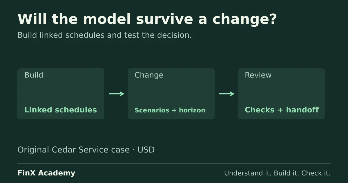
Define the decision, build traceable schedules and test changes before handing the model over.
Build a readable, testable financial model that another analyst can use. Nine free written lessons explain decision scope, model structure, monthly schedules, scenarios, circularity, checks and handoff. The original Cedar Service case includes an editable workbook, deliberate error diagnosis and horizon changes.
Prerequisites: Excel foundations and basic accounting for analysts. Reuse Excel for Financial Modeling for reference, switch and sensitivity drills. F06 adds the design and robustness work around those mechanics; full integrated three-statement modelling belongs to F07.
Download the practice workbook and complete source pack. Six of the 27 native IDE exercises are free. Formula grading is separate from self-reviewed design choices and the required written handoff.
1. Define the decision before the workbook
Outcome: specify a decision, output, boundary and time basis another analyst can challenge. Prerequisites: F02 formula fluency and basic F03 profit, cash and debt concepts.
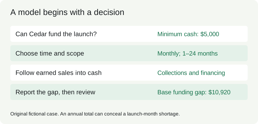
Cedar Service is considering a small new service line. The manager asks: “Can we launch with the proposed loan and retain at least $5,000 of cash?” That is more useful than “Build a model.” It tells us which outputs matter: the lowest forecast month-end cash, extra opening funding needed, operating contribution, closing debt and uncollected revenue.
Write a model brief before adding formulas. Name the decision owner, alternative, information cutoff, period, units and exclusions. Here the alternatives are launch or do not launch. The information cutoff is 9 October 2026. The forecast begins January 2027, uses monthly periods and defaults to twelve months, with one to twenty-four supported. All amounts are nominal USD, without scaling. Service units and dollars per service are different measures. Positive costs are subtracted from revenue or cash.
The case deliberately stops short of a complete valuation or three-statement forecast. It has revenue, collections, debt and cash schedules. It excludes income tax, depreciation, inflation, inventory, payables, terminal proceeds and a revolving facility. Monthly cash can hide a cash shortfall within the month. A positive contribution does not establish project value. Those limitations shape the recommendation, rather than belonging in a footnote nobody reads.
Worked design
Opening cash is $6,000. Equipment costs $24,000 at launch; the proposed loan provides $12,000 at the start of month one. Base demand begins at 120 services and adds ten per month, capped at 200. Each service sells for $100 and costs $40; monthly fixed cash costs are $3,000. Seventy-five percent of current sales is collected in the month, with the rest collected next month. These are fictional teaching facts and assumptions, not a real investment opportunity.
An annual total would miss the launch-month funding problem. Daily forecasts would imply timing evidence we do not have. Monthly detail is proportionate for this first decision, followed by a separate cash-timing review before committing funds. The launch switch applies to operations, equipment and the proposed new loan together. Existing opening balances remain existing balances.
Practice, hints and review
Write a five-line brief with one decision question, two alternatives, three outputs, a time basis and exclusions. Predict whether collecting revenue later changes contribution or cash.
Hint 1: begin with a decision the manager can take. Hint 2: distinguish total cash generated from the lowest balance. Hint 3: “Test whether the proposed launch stays above $5,000 at each month end; show the maximum funding deficit and its month.”
Reasoning and transfer
Later collection reduces early cash without changing earned revenue or contribution in this case. A horizon is a reporting choice, not an automatic liquidation date. A six-month result excludes months seven onward and retains receivables and debt outstanding at month six. Do not invent repayment or collection just because the forecast ends.
The numerical grader can check a funding calculation. It cannot decide whether $5,000 is an adequate cash floor, whether the demand forecast is credible or whether monthly resolution is sufficient. Those are design choices for review.
2. Separate evidence, assumptions, calculations and outputs
Outcome: trace an output to its drivers without overwriting source evidence. Prerequisite: lesson 1.
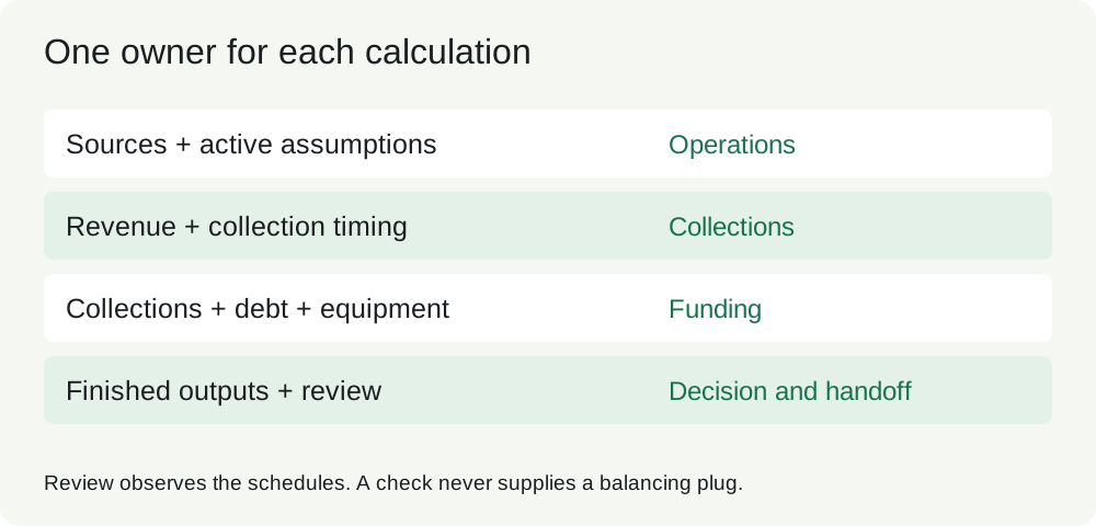
Four roles make a model readable. Sources preserve the supplied facts and their provenance. Assumptions contain forecast choices and controls. Schedules perform the business calculations. Outputs answer the decision. A check is a fifth, terminal role: it observes these areas and reports an inconsistency. It must not become an input that forces the model to agree with itself.
The workbook places Decision first, Assumptions next, then Operations, Collections and Funding. Sources and Review sit to the right. This physical order helps a reader; the calculation direction still runs from sources and active assumptions into schedules and outputs. A separate sheet is useful for each schedule here because linkage is a learning objective. A small single-purpose calculator can use labeled sections instead.
Build a source and assumption record
The original source pack identifies S1 opening balances, S2 equipment and capacity, and A1 management scenarios. Preserve an ID, description, unit, date and confidence limitation. A supplier quote and a management demand forecast are different evidence. Put the scenario price in Assumptions, not inside =Units*100. A constant such as twelve months per year is a labeled convention. Structural constants such as zero, one, or a row index are different from an undocumented commercial assumption.
Every column must use one unit. Here revenue equals service units multiplied by USD per service. The cash schedule uses USD. Costs and repayments are positive input amounts and cash outflows when subtracted. A negative closing cash balance means unfunded cash need before any additional financing; it is not an overdraft already obtained.
Use restrained formatting as a navigation aid. Editable financial inputs are blue on pale yellow, same-sheet formulas dark, cross-sheet formulas green, and decision outputs dark. The selected scenario is visible on every sheet. Color never substitutes for labels, a source record or access protection. The workbook is editable so learners can repair it; the color scheme does not lock cells.
Worked trace and practice
Trace closing cash from Decision to Funding, then to Collections, then to Operations, then to the active price and units. Explain why a signed −24,000 equipment assumption would be wrong when the cash formula already subtracts capex.
Hint 1: count sign changes. Hint 2: use positive 24,000 in Sources and subtract the capex row once. Hint 3: a double negative makes buying equipment appear to generate cash.
Solution and review boundary
A proper trace has one authoritative price for each period and one owner for each calculation. The output links to closing cash rather than recomputing all cash flows. A link to a local source cell avoids an external-workbook dependency. The handoff states that this workbook needs no external files, macros or refresh connections to recalculate.
A zero check can establish that signs implement a specified rule. It does not establish that the rule represents the actual contract. Reconcile the source and review its interpretation separately. For additional lookup and reference practice, reuse Excel for Financial Modeling; F06 focuses on how these mechanics work together.
3. Build a timeline that can change
Outcome: construct consistent monthly schedules and extend the reporting horizon without changing commercial logic. Prerequisite: lesson 2 and F02 references.
Give the forecast one period index and one start date. The first month is index one; the next is the prior index plus one. Use a true date for each month. EDATE(StartDate,Index-1) moves by calendar months, unlike adding thirty days. A visible active-period flag equals one when the index is within the selected horizon and zero otherwise. All schedules link to that timeline.
The supplied workbook prebuilds twenty-four months. Changing the horizon from twelve to six or eighteen changes which months contribute to outputs. It does not shift or erase the existing assumptions, accelerate collections, repay remaining debt, or add terminal proceeds. The twenty-four-month limit is explicit. Extending beyond it requires extending every schedule, output range and check range and rerunning the tests; changing a validation limit alone is insufficient.
Use one formula pattern
For month t, demand is initial demand plus (t-1) × monthly additions. Sold units are the lower of demand and capacity, multiplied by the launch switch. Revenue is units times price. Variable costs are units times unit cost. Operating contribution is revenue less variable and fixed costs. Do not round the underlying economics just to make the displayed table look tidy.
In the Base case, months one, two and nine sell 120, 130 and 200 services. Revenue is $12,000, $13,000 and $20,000. Month ten still sells 200 because capacity binds. A growth formula copied beyond capacity without the minimum rule would overstate both revenue and cash.
Use the same column for the same month across Assumptions, Operations, Collections and Funding. Anchor global control cells; let period-specific driver columns move. Inspect the first, middle and final supported month, and the first newly activated month after a horizon change. A correct first formula does not prove that copying worked.
Practice and extension
Write the first two month dates and the demand, units, revenue and contribution formulas. Change Base price from $100 to $110. At 120 units, month-one revenue rises $1,200; variable costs do not change, so contribution also rises $1,200. Restore the price. Now change only month eighteen’s price: months one through seventeen must remain unchanged.
Hint 1: the time index and capacity rule are independent. Hint 2: distinguish a shared scalar from a period-specific driver. Hint 3: use the current column’s active price, rather than a fixed link to month one.
Horizon solution and common mistakes
A flow such as revenue is summed over active months. A stock such as debt uses the balance in the last active month. Summing monthly closing debt gives no meaningful closing balance. A minimum cash calculation must exclude inactive zero placeholders, or it will show an artificial low after the selected horizon.
The starter leaves four selected first-month formulas blank. Complete them before using the decision output. The remaining formulas demonstrate the copied pattern. For independent assessment, build the schedules in a new workbook using the source pack and compare only after saving your attempt. Formula consistency is partly automatable; the choice of monthly grain and the twenty-four-month support limit requires review.
4. Switch assumptions without hiding hardcodes
Outcome: run coherent scenarios and controlled sensitivities through the same model. Prerequisite: lesson 3.
A scenario changes a related set of assumptions. A sensitivity changes one specified input while holding the others fixed. Neither is a separate spreadsheet whose formulas quietly evolve away from the original. The model has one case selector: 1 Base, 2 Downside, 3 Upside. Each driver has an Active row above its three case rows, sharing the same monthly columns. Every schedule reads Active, never a particular case row.
| Assumption | Base | Downside | Upside |
|---|---|---|---|
| Initial services per month | 120 | 90 | 140 |
| Added demand per month | 10 | 5 | 15 |
| USD per service | 100 | 95 | 105 |
| Variable USD per service | 40 | 42 | 39 |
| Fixed USD per month | 3,000 | 3,300 | 3,000 |
| Current-month collection | 75% | 60% | 85% |
Case selection can use CHOOSE over validated inputs. Validate both the selector and the selected assumption. Blank is unknown; zero can be valid. A missing Downside price must leave Base usable, then show an unavailable result when Downside is selected. Never use IFERROR(...,0) to hide the defect. A pasted value can bypass a dropdown, so the formulas also validate control values.
Scenario exercise
Save the Base results. Select Downside and explain the path from lower price and slower collections to cash. Return to Base and confirm the initial results. Then use the launch switch: zero turns off new operations, equipment and the proposed loan. Opening balances remain. A switch needs a documented business meaning, not a label such as “option on” with unclear effects.
Sensitivity exercise
Use a change–recalculate–record–restore process in the Review log. Record scenario, horizon, exact changed cells, old/new values and the resulting cash output. Start with Base, twelve months. Change collection from 75% to 50% in all active months. Month-one collections fall from $9,000 to $6,000, and the opening funding requirement rises by $3,000. Operating contribution stays the same. Restore all affected cells and verify the baseline.
The log contains learner-recorded snapshots, explicitly labeled as such. They are not live scenario outputs. Do not use a saved comparison after changing assumptions without rerunning it. Existing Excel sensitivity grids teach mixed-reference mechanics; this case adds linked dependencies and a reproducible test log. A native Excel What-If Data Table is optional further practice, not a claimed browser-graded feature.
Hints: identify the one selector; trace an Active driver into each schedule; predict the direction before recalculating. Transfer: increase price while reducing demand. Explain why an isolated price sensitivity may be less realistic than a coherent scenario. No formula check can certify that the chosen scenarios span the business’s actual risks.
5. Link schedules and document circularity
Outcome: build one-way dependencies and explain the chosen interest and financing method. Prerequisite: lesson 4 and basic F03 receivables and debt.
Operations supplies earned revenue. Collections supplies cash received and closing receivables. Funding supplies debt, interest and cash. Decision reads finished outputs. Review observes each schedule independently. This dependency map makes it possible to investigate a bad result upstream without rebuilding it in every sheet.
Collections schedule
Opening receivables plus sales less collections equals closing receivables. The case collects all opening receivables and the current-month share of sales. In month one, opening receivables are zero, sales are $12,000 and collections are $9,000. Closing receivables are $3,000. Month two collects that $3,000 plus 75% of $13,000, or $12,750. Closing receivables are $3,250. There are no write-offs, taxes on invoices, or multi-month arrears in this simplified policy.
Debt and cash schedule
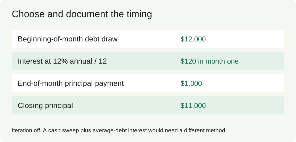
Opening debt plus new draw less repayment equals closing debt. The $12,000 draw occurs at the beginning of month one. Repayment occurs at month end and is capped at available principal. Interest is (opening debt + beginning-of-month draw) × annual rate ÷ 12. At 12%, month-one interest is $120 and month-two interest is $110. The full-year total is $780. No interest is charged after principal reaches zero.
Cash then equals opening cash plus collections, less variable and fixed payments and capex, plus draw, less repayment and interest. Negative forecast cash remains visible. The model reports required additional opening funding, but does not insert that funding automatically into the cash schedule. It is a decision output, not a balancing plug or a loan commitment.
What would create a loop?
If debt repayment depended on closing cash after interest, and interest depended on average closing debt after that repayment, the calculation would feed back into itself. Switching on iteration can make a workbook return a number without establishing convergence or economic correctness. Microsoft documents both circular-reference diagnostics and iterative calculation in Excel support.
F06’s policy is no intentional circular references; iteration off; beginning-of-month debt interest; fixed end-of-month principal repayment. This is an explicit timing convention, not a mathematically equivalent substitute for average-debt interest. Do not replace the convention silently. If the contract requires a different method, redesign the schedule and document it. F07 handles integrated statements and more complex funding needs.
Practice and review
Calculate months one and two of receivables, debt and interest. Trace each opening balance to the preceding closing balance. Then draw the proposed cash-sweep loop on paper and identify which assumption makes it circular.
Hint 1: distinguish a forward link from a feedback link. Hint 2: starting debt and a known draw are already available before interest. Hint 3: the cash shortfall should remain an output until financing is separately decided.
The reviewer checks the timing convention against the intended economics. Formula tests check its implementation. A future intentional iterative model must document its loop, initialization, iteration limit, tolerance, convergence tests and failure behavior, including save/reopen and stressed inputs. This workbook does not claim to implement or verify that future method.
6. Design checks before finishing the model
Outcome: distinguish an incomplete build, a failed numerical control and a design issue requiring review. Prerequisite: lesson 5.
Write a check register while the model is still a blank plan. Specify each risk, calculation, expected result, tolerance and repair path. “The model balances” is too vague. A copied error can balance with itself. Use independent identities and compare upstream drivers with downstream results.
| Risk | Control | Interpretation |
|---|---|---|
| Wrong revenue driver | Revenue less units × active price | Zero within $0.000001 |
| Collections timing error | Opening AR + sales − collections − closing AR | Zero within tolerance |
| Debt sign or repayment error | Opening debt + draw − repayment − closing debt | Zero within tolerance |
| Wrong interest timing | Interest less (opening debt + draw) × rate ÷ 12 | Zero within tolerance |
| Cash sign or omitted flow | Closing cash less independently reconstructed cash | Zero within tolerance |
| Truncated output range | Displayed ending balance less last active closing balance | Zero within tolerance |
| Incomplete construction | Required numeric result count | Missing cells remain visible |
Checks live in Review and do not feed the business model. The schedules guard their own missing inputs so that an incomplete build cannot masquerade as a valid zero. Review reports missing, failed and passed controls separately. Never convert an unavailable check to zero just to produce a clean summary. Review also tests timeline coverage and continuity.
Deliberate errors
After completing the four blank starter formulas, save a clean baseline. Make one fault at a time. First, draw a hypothetical loop on paper: collections depend on closing receivables, while closing receivables are calculated from opening receivables plus sales less collections. Explain why this is circular; do not enable iteration. Our workbook independently calculates closing receivables from uncollected sales, so it has no such cycle. Now plant a numerical timing fault: change month-two collections to current sales times the collection rate only: it omits the $3,000 opening balance.
Next, change month-one cash to add capex. The cash control must expose a $48,000 error. Finally, make Decision’s ending cash link stop at month twelve, then change the horizon to eighteen. The output-link control must fail. Repair the actual formulas; do not change expected controls to accommodate the mistakes.
One subtler fault is to type today’s correct revenue as a number. An equality check may pass today. Change price and see it fail, then restore both formula and input. This is why changed-input tests complement point-in-time reconciliations. A formula-presence scan is useful but does not prove the formula is appropriate.
Practice, hints and review
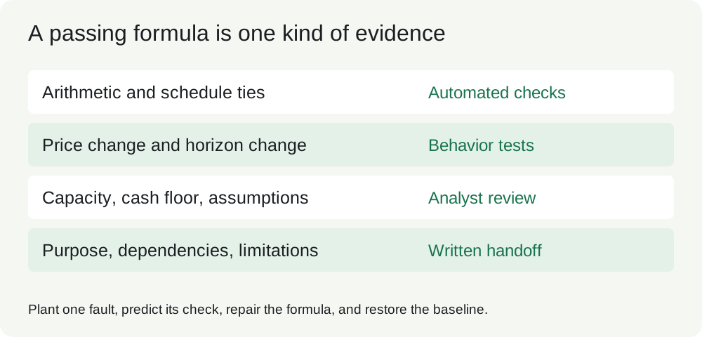
Before injecting each error, write which check should fail and the expected difference. After repair, rerun the baseline and at least one changed input. Hint: two errors with opposite signs can cancel at the grand total, so inspect monthly detail and gross exceptions.
A wrong but consistently applied demand forecast can pass every arithmetic check. Independent source credibility, capacity adequacy, cash floor, missing taxes, and monthly timing remain analyst review items. The workbook provides separate written fields for these questions. A populated field establishes completion of a response, not its quality or approval.
7. Review the model as the next analyst
Outcome: deliver a readable workbook with a reproducible change log and concise handoff. Prerequisite: lesson 6.
Start the review at Decision. The manager should see the question, selected scenario, horizon, key outputs and limitations without searching through a wall of formulas. Then follow one output back through the schedules to evidence. Check units, signs, chronological columns, comparable row positions, clear inputs and sufficient number precision. Do not hide rows containing overrides or unexplained plugs.
Review formulas at boundaries: the opening period, a typical middle month, month twelve when debt finishes, the capacity threshold, and the last supported month. Compare the formula pattern across each row. First-period opening balances and one-time launch spending are legitimate exceptions when documented. A pasted number in the middle of a formula row is not explained by matching the current answer.
Save a useful version
Use a dated version such as cedar-model-v1.0-2026-10-09.xlsx. Record what changed, who prepared it, who reviewed it, the source version, the case and horizon tested, and outstanding issues. Keep a clean baseline before error diagnosis. A filename containing “final-final” does not identify what was verified. Do not claim review by another person unless it occurred.
The workbook’s Review sheet includes editable fields for purpose, inputs, dependencies, limitations, circularity policy and review conclusion. These are separate from the source notes and formula checks. The source pack contains a blank handoff template and a clearly labeled reference handoff. Save your own answer before reading the reference.
Example handoff structure
“Purpose: assess whether Cedar’s proposed launch retains $5,000 at every forecast month end. Inputs: S1 opening balances, S2 equipment/capacity and A1 scenario assumptions. One selector controls all Active assumptions; launch controls incremental operations, capex and the proposed loan. Dependencies: Operations → Collections → Funding → Decision. No external workbook links, macros or live connections. Limitations: monthly timing, no taxes, inventory, payables, terminal value or automatic financing. Circularity: iteration off; interest uses opening debt plus beginning-of-month draw, with principal paid at month end. Tested: baseline, scenarios, six/eighteen-month horizons, input changes and repaired faults. Recommendation and unresolved evidence: state these explicitly.”
Practice and reviewer rubric
Give a colleague the workbook and your handoff. Ask them to change the case, explain the funding result and return to baseline without your help. If you work alone, close the file and repeat later using only your written notes; label this self-review. Do not call it an independent review.
Hint 1: define the purpose before listing sheet names. Hint 2: mention each dependency that could prevent recalculation. Hint 3: state the interest timing and missing funding mechanism explicitly.
Assess four categories separately: numerical implementation, behavior after changes, model design, and explanation quality. Automated checks cover specified formulas and reconciliations. A reviewer evaluates whether the model answers the right question with adequate evidence and appropriate limitations. The free written course and downloadable reference solutions are teaching materials, so this case is not an unseen professional certification.
8. Test changes and repairs systematically
Outcome: reproduce a small test matrix and explain what each test detects. Prerequisite: lesson 7.
Robustness means preserving the stated model relationships when supported inputs change. It does not mean accepting every possible number or extending indefinitely. The supported horizon is one to twenty-four whole months. The case selector is one, two or three. Launch is zero or one. Collection percentages must be between zero and one; blank active drivers are invalid. Every test starts from a recorded clean baseline and restores it afterward.
| Test | Expected behavior | Risk addressed |
|---|---|---|
| Base → Downside → Upside → Base | All schedules change, then baseline returns | Partial scenario wiring |
| Horizon 12 → 6 → 18 → 24 → 12 | Flows and ending stocks use active months | Fixed output ranges |
| Base price 100 → 110 in month one | Revenue/contribution +1,200; collections +900 | Hidden commercial hardcode |
| Collection share 75% → 50% | Earlier cash falls; contribution unchanged | Cash versus revenue confusion |
| Launch 1 → 0 | New operations/capex/loan stop together | Incomplete switch |
| Active price blank | Dependent results unavailable | Missing input treated as zero |
| Unselected case price blank | Active case still calculates | Overbroad input gate |
| Price zero | Valid zero revenue; costs remain | Zero confused with missing |
| Horizon 0, 25 or 6.5 | Explicit invalid control | Unsupported extension |
Diagnose a copied number
Complete the starter and set Base, twelve months. Replace month-one revenue with the current numeric result, $12,000. The revenue reconciliation will still be zero. Now change month-one price to $110. The copied number stays at $12,000, while units times price is $13,200. The control difference becomes −$1,200. Restore the formula, confirm $13,200, then restore price to $100 and confirm the baseline again.
Diagnose the horizon
Link ending cash directly to month twelve. At the default horizon, it appears correct. Select eighteen months. The model’s output-link check must compare the displayed result with the last active month and flag the stale link. Restore the dynamic INDEX selection. Shorten to six months too: extending is only half the test. Confirm remaining debt and receivables stay outstanding rather than disappearing at the horizon.
Document the evidence
For each test record starting version, input cells, old/new values, prediction, observed result, check triggered, repair and baseline restoration. “Tested scenarios” without cases, outputs or expected relationships cannot be reproduced. Inspect the workbook at readable zoom and after reopening in your intended spreadsheet application. Export/recalculation QA in a compatible engine is not proof of every native Excel feature or application setting.
Hints: change one thing at a time; test a boundary as well as a typical value; use an independent arithmetic expectation. Transfer: a model has correct formulas but assumes all customers pay within one month. Name evidence needed before trusting its funding estimate. Formula tests cannot establish customer behavior.
9. Case: construct, explain and hand off the Cedar model
Outcome: build a decision model, change it safely and explain its limitations. Prerequisites: lessons 1–8; F02 and basic F03.
Download the practice workbook and source pack. The workbook supplies a readable architecture, controls, linked schedules and four blank first-month formulas. Start there for a guided attempt. For the independent build, start from a new workbook and the source pack, preserving your attempt before consulting the reference solution. The source pack contains public teaching answers, so this is a practice assessment.
Construction brief
Decide whether launching the service line with the proposed financing preserves a $5,000 month-end cash floor. Model monthly periods from January 2027, initially twelve months, with support for one to twenty-four. Use USD, positive expenses and repayments, a 200-service capacity and the three supplied cases. Keep sources, assumptions, calculations, outputs and terminal checks distinct. Use one scenario selector and the documented launch switch.
Build Operations, Collections and Funding in sequence. Link period columns and opening balances consistently. Interest applies the annual rate to opening debt plus a start-of-month draw, then divides by twelve; principal is paid at month end and never exceeds principal available. The model reports cash before additional funding. It must show a funding gap rather than manufacture a cash plug.
Design the check register first. Include revenue-driver, receivables, debt, interest, cash, timeline and output-link checks. Then complete the starter’s first-month units, collections, interest and closing cash. Each incomplete dependency must remain visible. The IDE drills check component formulas; the workbook and written assessment test the complete model architecture.
Required change and repair tasks
Run all three scenarios. Change the horizon to six, eighteen and twenty-four, then return to twelve. Change price and collection timing, and test launch zero. Clear a selected driver, then an unselected driver; show different consequences. Record predictions and observed outputs.
Inject three numerical faults separately: omit opening receivables from month-two collections; add instead of subtract month-one capex; and freeze the ending-cash output at month twelve before extending to eighteen. Record each failing check, repair the formula and prove restoration. Also replace a revenue formula with its current numeric answer and use a price change to reveal it. Explain a potential debt-interest circularity without leaving an active cycle in the submitted file.
First-month worked solution
Base sells 120 services for $12,000. Variable costs are $4,800 and fixed costs $3,000, leaving $4,200 contribution. Collections are $9,000 and closing receivables $3,000. Debt draw is $12,000, repayment $1,000, interest $120 and closing debt $11,000.
Closing cash is 6,000 + 9,000 − 4,800 − 3,000 − 24,000 + 12,000 − 1,000 − 120 = −5,920. The gap to the $5,000 minimum is $10,920. Positive operating contribution does not remove the launch-month funding requirement. The model assumes no extra funding has yet been committed.
Omitting month-two opening receivables reduces collections and cash by $3,000 if receivables remain independently calculated. Adding $24,000 capex instead of subtracting it overstates cash by $48,000. A fixed twelve-month output fails only when the horizon changes. A correct numeric hardcode can pass today’s equality check and fail the changed-price test.
The source pack’s solution.json supplies independently calculated monthly schedules for each case and supported test horizon. Compare after saving your attempt; inspect the calculation path whenever results differ.
Required short handoff and assessment
Write 150–250 words covering purpose, inputs, dependencies, limitations and circularity policy. State the recommended next action, the cash requirement and the evidence still needed. Identify the version and tests run. A defensible conclusion is to defer commitment until funding and within-month payment timing are resolved; do not turn the calculation into an unconditional investment recommendation.
Numerical and changed-input checks are automated where stated. Scope, input credibility, time resolution, cash floor, scenario adequacy, circularity convention and handoff quality require self-review or a named human reviewer. A passed formula exercise does not approve those choices. Continue to F07 for the integrated income statement, balance sheet and cash-flow forecast.
Sources and further reading
All company facts, quotes and forecasts are original fictional teaching data. Prepared 9 October 2026 for a January 2027 start. Units are USD, service units and USD per service. Positive expenses and repayments are subtracted. Monthly demand is initial demand plus cumulative linear additions, capped at capacity. No compounding is implied.
S1 provides opening cash, debt and receivables. S2 provides equipment paid at launch and operating capacity. A1 is a management scenario assumption, not a disclosed result. A2 is the proposed financing: 12,000 drawn at the beginning of month one if launch is on, 1,000 repaid at each month end, 12% annual interest divided by twelve on opening principal plus the draw. No debt sweep or cash plug. Opening balances are not switched off.
The model excludes taxes, depreciation, inventory, payables, defaults, seasonality, terminal value and intra-month timing. The horizon does not liquidate the business. Uncollected invoices and unpaid debt remain at the last forecast date. The reported extra opening funding is a liquidity requirement, not assumed proceeds or project NPV.
Optional primary references checked 9 October 2026: ICAEW modelling principles, FAST Standard, Microsoft circular references. These inform general practice; the Cedar architecture, assumptions and cases are original.
Build and stress-test the Cedar model
Start with six free exercises on scope, layers, units and signs. Continue with timeline design, scenario switches, linked schedules and error diagnosis in full access. Review design choices and the written handoff separately.
Continue with guided practice
Build a readable decision model, test changed assumptions and review its design and handoff.
Model architecture and construction course