Excel foundations and formula fluency: a free course

Build a financial worksheet that still works after its inputs change. This free course starts with cells and number formats, then teaches references, logic, conditional totals, lookups, dates and a complete sales-file case.

Start here: you need basic arithmetic and the units covered in financial numeracy. The nine lessons include worked examples and public solutions. Native Excel is needed for the optional Table, PivotTable, chart and export labs; those actions are self-reviewed separately from browser formula exercises.

Download the editable practice workbook. All Northstar data is fictional. Keep the raw source intact, attempt each task before opening its answer, and record the changed-input checks.

1. Find your way around a worksheet

A sales report shows 30% beside a bottle price. Did the price fall, or did someone apply the wrong number format? Before writing a formula, learn to distinguish what a cell stores from how it looks.

Outcome: navigate a workbook, enter a linked calculation and choose a display that preserves its meaning. Prerequisite: multiplication and the units covered in F01. Our fictional company, Northstar Bottles, sells bottles and accessories. The examples are original practice data, not company disclosures.

A workbook has sheets; a sheet has cells

A workbook is the file. Sheets are the named tabs inside it. Columns use letters and rows use numbers, so C5 means column C, row 5. C5:C8 is the four-cell vertical range from C5 through C8, including both endpoints. The active cell receives your typing. The formula bar shows its stored value or formula.

Create a sheet called Sales practice. Enter these labels and values:

Cell	Entry	Meaning
B3	Units sold	Label
C3	120	Number of bottles
B4	Price per bottle (USD)	Label
C4	30	Dollars per bottle
B5	Revenue (USD)	Label
C5	=C3*C4	Formula, returning 3,600

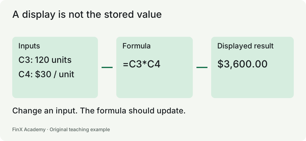
Click C5 and inspect the formula bar. You should see =C3*C4, even though the grid displays 3,600. Change C3 to 125. C5 should change to 3,750. Undo the change. A typed 3,600 would look right initially but would not respond to the new units. This changed-input check is your first formula audit.

Use the name box to select C5 directly. Select C3:C5, copy it, and practice pasting into a spare area. Undo afterward. Copying a formula and pasting its value are different actions: a value paste takes a snapshot and breaks the calculation link. Keep a source copy before experimenting with destructive edits.

Store the value; format the display

Enter 0.125 in C7 and apply a percentage format with one decimal. The display becomes 12.5%; the underlying value remains 0.125. Entering 12.5 and then applying that format displays 1,250%. Formatting does not divide the stored number by 100.

Enter 12.345 in C8 and show two decimals. Excel displays 12.35, but a formula that refers to C8 still uses 12.345. Use ROUND only when the calculation itself needs a rounding rule, such as line-item invoice cents. Lesson 3 explains that distinction.

Identifiers are different from quantities. Product code 0012 may need to stay text so its leading zeros survive. A quantity of twelve should normally be numeric. Do not convert every text field to numbers just because it contains digits. A number stored as text may be ignored by a range sum or fail an exact lookup against a numeric key.

Work efficiently without hiding mistakes

Use the keyboard for repeatable actions, but understand each action first. On Windows, Ctrl+C/Ctrl+V copy and paste, Ctrl+Z undoes, and Ctrl+arrow moves to a data-region edge. On Mac, use the corresponding menu command or shortcut shown in the application. Browser and operating-system shortcuts can intercept keys; a keyboard shortcut is not an assessed finance competency.

Keep one header row, readable column widths and explicit units. Freeze a long table’s header when scrolling would hide it. A #### display can mean the column is too narrow; inspect the stored value before changing the data. Never make a report fit by removing its currency or period labels.

Practice and check

Build the small worksheet example, then use 80 bottles at $25. Predict the answer before changing the sheet. Inspect whether the output contains a formula. Next, display 0.075 as a percentage and 1,234.567 as dollars with two decimals.

Answers and reasoning

Revenue is $2,000. The displays are 7.5% and $1,234.57. The stored amount in the last cell is still 1,234.567. If revenue does not update, check whether you pasted a value, entered the formula as text, or changed the wrong input.

Transfer: create the same calculation on a new sheet without copying the original. Explain which entries are labels, inputs and formulas, and why a screenshot cannot establish that the calculation updates.

2. Copy formulas without moving the wrong input

Northstar applies one 10% discount to three orders. The first formula works. The next one returns the full gross amount because copying it moved the discount reference into an empty cell. The problem is the reference, not multiplication.

Outcome: choose relative, absolute and mixed references from the relationship the formula represents. Prerequisite: lesson 1.

Decide what should move

Put the discount in C3 as 0.10. In B6:B8 enter order labels, and in C6:C8 enter gross sales of 300, 450 and 600. In D6 enter =C6*(1-$C$3), then fill down through D8.

Output	Formula after filling	Net sales (USD)
D6	=C6*(1-$C$3)	270
D7	=C7*(1-$C$3)	405
D8	=C8*(1-$C$3)	540

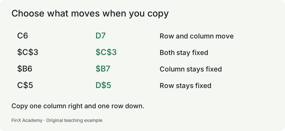
Each row needs its own sales amount, so C6 changes to C7 and C8. Every row shares the one discount, so $C$3 stays fixed. A dollar sign locks the coordinate immediately after it during copying. It does not protect the cell from editing or make the business assumption correct.

Reference	Copy one column right and one row down	What stays fixed
C6	D7	Nothing
$C$6	$C$6	Column and row
$C6	$C7	Column only
C$6	D$6	Row only

Do not memorize dollar signs without considering the layout. If every month has a different discount in row 3, =C6*(1-C$3) is appropriate when filling across months. Locking $C$3 in that layout would incorrectly apply the first month’s assumption forever.

A two-dimensional calculation needs two different anchors

Build a price-volume grid. Put quantities 100 and 200 in B6:B7, and prices $20 and $30 in C5:D5. In C6 use =$B6*C$5. Fill across and down.

Units / price	$20	$30
100	2,000	3,000
200	4,000	6,000

The unit count always comes from column B but changes by row. The price always comes from row 5 but changes by column. D7 should therefore contain =$B7*D$5. Inspect the first, middle and last copied formulas. One correct corner does not validate a grid.

Link across sheets deliberately

='Assumptions'!$C$3 reads C3 from the sheet named Assumptions. Single quotes support names containing spaces. A link to another workbook adds a dependency on that file and its availability. For these lessons, keep the inputs in the same workbook and label them rather than creating unnecessary external links.

Copying, cutting and inserting rows are not interchangeable operations. This lesson’s reference table describes copying. After moving or restructuring a model, inspect the affected links again. If a formula depends on itself, directly or through other cells, you have a circular reference; redesign the dependency rather than enabling iteration to silence the warning.

Check behavior, not just the displayed answer

Change the shared discount to 20%. The three net sales should become 240, 360 and 480. Restore 10%. Then change only the second order to 500: only its net sales should become 450. This tests both the shared input and the row-specific input.

A grader may accept mathematically equivalent formulas. Some single-cell graders ignore dollar signs when comparing formulas. That does not prove a formula is safe to copy. The desktop fill-and-change task assesses reference behavior directly; record it separately from a numerical exercise pass.

Practice and check

1. Copy =C6*$C$3 from D6 into E7. What does it become?
2. Put monthly volume in row 8 and each month’s price in row 4. What formula in C9 should copy across correctly?
3. Repair a grid that uses =$B$6*$C$5 in every cell.

Answers and reasoning

1. =D7*$C$3.
2. =C8*C4 works for a single revenue row. =C8*C$4 also supports copying down when row 4 must stay the price source.
3. Use =$B6*C$5 at C6, then fill. Fix the unit column and price row while allowing the relevant coordinate to change.

Transfer: add a third price and third quantity. Predict the new bottom-right result, fill the formulas, and change one header to prove the new outputs use the intended input.

3. Calculate, make a decision and expose errors

A cell can contain a valid formula and still answer the wrong question. =300-180/300 calculates 299.4. Northstar’s gross margin is 40%. Parentheses express the business relationship.

Outcome: use arithmetic, SUM, IF and deliberate error handling without concealing missing data. Prerequisite: lessons 1–2 and F01 percentages.

Start with the equation

Put revenue of 300 in C3 and cost of sales of 180 in C4. Gross profit in C5 is =C3-C4, or 120. Gross margin in C6 is =C5/C3, or 40%. The equivalent single expression is =(C3-C4)/C3. Multiplication and division occur before addition and subtraction unless parentheses change the grouping.

Use =SUM(C8:C10) to add detail values 270, 405 and 540, giving 1,215. If C11 already contains their subtotal, summing C8:C11 counts the detail twice. A formula’s range is part of its meaning. SUM also does not prove that all expected inputs are numeric and present; a text quantity can disappear from a range total.

IF expresses a rule with a boundary

Suppose shipping is free when order value is at least $100. With order value in C3, shipping fee in C4 and threshold in C5, use =IF(C3>=C5,0,C4). At exactly 100, shipping must be zero. A condition using > would fail that boundary.

Test 99.99, 100 and 100.01. For a rule that requires both a minimum spend and approval, use AND inside IF. For a rule allowing either qualifying condition, use OR. Write the policy in words first so the formula’s condition can be checked against it.

Zero and missing are different

If verified revenue is zero, margin is not defined by division. One explicit presentation rule is =IF(C3=0,"n.a.",C5/C3). This assumes C3 and C5 have already been validated as numeric. A blank input must not quietly become the same case as a genuine zero. Use ISNUMBER or an input check to distinguish the two before calculating.

Returning text such as "n.a." makes the exception visible, but a downstream SUM can ignore that text. A total of the remaining rows may then look complete. Keep an exception count next to a report whenever omitted values would matter. Do not publish a complete margin comparison while one required input is missing.

Read errors as clues

Error	First investigation
#DIV/0!	Is the denominator zero or blank?
#N/A	Is the lookup key absent or of the wrong type?
#VALUE!	Did text enter a numeric operation?
#REF!	Was a referenced cell or range removed?
#NAME?	Is the function/name misspelled or unsupported?

IFERROR(expression,fallback) catches many different errors. It is useful when the fallback is justified for all of them. Wrapping a whole report in IFERROR(...,0) can turn a deleted input range into apparently real zero revenue. For a missing lookup, use the lookup’s not-found option or IFNA after investigating the cause. For an expected zero denominator, test that condition explicitly.

Decide where rounding belongs

Suppose each of three invoice lines is 0.335 dollars before rounding. If the contract rounds each line to cents, each becomes 0.34 and the invoice total is 1.02. If the agreement rounds only the aggregate, 1.005 rounds to 1.01 in the stated decimal calculation. Those are different policies. Excel uses binary floating-point arithmetic, so test values near a rounding boundary in the intended spreadsheet engine rather than assuming every decimal behaves exactly.

For a straightforward exercise, 19.995 rounded to two decimals is 20.00 in Excel. ROUND(C3,2) changes the calculation result; a two-decimal number format changes only its display. Keep intermediate precision unless a business rule calls for rounding at that step.

Practice and check

Calculate gross profit and margin for revenue of 500 and cost of sales of 350. Then implement a fee of $8 below a $100 threshold. Test a zero denominator and a missing input separately. Explain why replacing both with a numerical zero would be misleading.

Answers and reasoning

Gross profit is 150 and margin is 30%. The fee is 8 below 100 and 0 at or above 100. A zero denominator makes the ratio undefined; missing data means the ratio cannot yet be determined. Neither establishes a zero margin.

Transfer: repair a report containing IFERROR(...,0). Identify the specific error, correct its cause if supported by the source, and leave an explicit exception when the necessary input is unavailable.

4. Summarize the rows that answer your question

Northstar wants North-region shipped sales, not every North order. A regional total can be arithmetically correct and still include a canceled order. Translate the question into conditions before choosing a function.

Outcome: use SUMIFS and COUNTIFS with aligned ranges, explicit criteria and independent reconciliation. Prerequisite: lessons 1–3.

A small table makes the rule visible

Place headers in B4:D4 and these five rows in B5:D9:

Region (B)	Status (C)	Revenue USD (D)
North	Shipped	300
South	Shipped	360
North	Shipped	450
North	Cancelled	225
South	Returned	-90

=SUMIFS(D5:D9,B5:B9,"North",C5:C9,"Shipped") returns 750. SUMIFS starts with the values to add, followed by pairs of condition ranges and criteria. Every included row must satisfy every pair. Check it independently: only 300 and 450 qualify.

=COUNTIFS(B5:B9,"North",C5:C9,"Shipped") returns 2. COUNTIFS counts matching rows; it does not count distinct customers or orders unless your source has exactly one row per customer or order. State the row grain before interpreting the count.

Build a summary that can be copied

Put region labels in F5:F6 and the required status in G3. In G5 use =SUMIFS($D$5:$D$9,$B$5:$B$9,$F5,$C$5:$C$9,G$3). Copy down. Source ranges stay fixed; the region changes by row. If you add more status headers across row 3, the mixed status reference moves across while keeping the header row.

Keep all condition ranges aligned with the sum range. D5:D9 paired with B6:B10 describes different records. Some range-size mistakes produce errors; a shifted range of the same size can silently return the wrong answer.

Operators need quoted criteria

To sum positive revenue use a criterion such as ">0". To compare against a threshold in G2, join the operator to the cell: ">="&G2. For a month, use two date conditions: on or after its first day, and before the next month’s first day. Lesson 6 gives the complete formula.

SUMIFS conditions use AND logic. To include Shipped or Returned, add two disjoint SUMIFS results, or create a documented eligibility column. Do not add overlapping conditions without considering double-counting. In the table above, shipped revenue is 1,110, returns are -90 and eligible net revenue is 1,020. Including the canceled row would incorrectly give 1,245.

Zero is not proof of source coverage

A SUMIFS result of zero may mean no records matched. It may also mean actual sales and returns offset each other. A matching COUNTIFS helps distinguish those cases, although a positive count still does not prove the amounts are numeric or the source complete. If a region should be present but its count is zero, investigate spelling, spaces, data types and the date range.

Reconcile the sum of all mutually exclusive regional totals to the eligible source total. This checks coverage of the summary categories. It cannot detect a duplicate that appears in both calculations, so the duplicate check remains separate.

Practice and check

1. Calculate South shipped revenue and its row count.
2. Calculate North revenue excluding the canceled row.
3. Explain why a sum for East of zero does not establish that East sold nothing.

Answers and reasoning

1. 360 and 1.
2. 750. In this sample, North has no returned rows.
3. East has no records in the supplied table. The source may omit the region. Check the source’s intended coverage before labeling zero as a business result.

Transfer: add a North return of -60. The North eligible total should fall to 690, while North shipped revenue remains 750. Extend every bounded range to include the new row and prove both behaviors.

5. Look up a value without trusting an ambiguous key

Northstar’s product list contains two prices for code B. XLOOKUP returns one without displaying an error. A successful match does not establish that the source has one correct answer.

Outcome: choose an exact-match lookup, diagnose missing matches and check duplicate keys before retrieving a value. Prerequisite: lessons 2–4.

Three ways to retrieve one price

Put product codes A, B and C in B5:B7 and prices 30, 45 and 20 in C5:C7. Put the requested code B in F3. These formulas all return 45 for this unique, complete mapping:

Method	Formula
XLOOKUP	=XLOOKUP(F3,B5:B7,C5:C7,"Unmapped",0)
INDEX and MATCH	=INDEX(C5:C7,MATCH(F3,B5:B7,0))
VLOOKUP	=VLOOKUP(F3,B5:C7,2,FALSE)

XLOOKUP searches the key range and returns the corresponding value. The explicit zero requests an exact match. INDEX retrieves a value by position; MATCH with zero finds the exact key’s position. VLOOKUP searches the first column of its table and returns the second column. FALSE is essential for an exact product-code match. Do not use approximate matching on an unsorted code list.

XLOOKUP is unavailable in Excel 2016 and 2019. INDEX/MATCH supplies the compatibility route. Feature availability in Excel does not establish support in another spreadsheet engine; the native labs name Excel as their target, while browser exercises use functions separately checked in FinX.

A lookup is a join with a relationship

Before retrieving the price, calculate =COUNTIFS(B5:B7,F3). A valid unique product mapping should produce 1. Zero means absent; more than one means ambiguous. A product master expects one row per product code. A sales table often has many rows per product, so use SUMIFS to aggregate those sales rather than taking its first match.

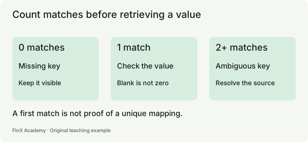
Add a second B with a price of 47. A first-match lookup may still return 45. Reversing source order can change the answer. Choosing the last match does not solve the business ambiguity. Ask whether the table needs an effective date, currency, region or other key. A duplicate with identical prices still needs a documented policy; the lookup does not establish that the duplication is harmless.

Missing data is not a zero price

For an unknown code X, XLOOKUP’s not-found argument can return "Unmapped". INDEX/MATCH can be wrapped in IFNA to identify an absent match. Do not automatically replace an absent price with zero. That would make an unpriced sale look free and understate revenue.

A found key with a blank price is another problem. A lookup may return a value that looks like zero, so check the mapped field too. For this lesson’s numeric prices, first confirm one key match, then validate that its source price is numeric. A legitimate price of zero and a missing price are different states. Keep affected rows visible in an exception list, and do not allow an aggregate to ignore text exceptions silently.

Diagnose a failure in a useful order

Inspect whether the key exists; compare the key’s type and length; inspect spaces or nonprinting characters; verify source and return ranges are aligned; then check duplicates and the returned field. The string 0012 and numeric 12 may refer to different identifiers. Converting both to numbers without a mapping policy can merge distinct products.

Practice and check

1. Use all three lookup methods to retrieve C’s price.
2. Request X and state what information is missing.
3. Add another B at 47 and write the question you would ask the source owner.

Answers and reasoning

1. 20 with the unique mapping above.
2. X has no mapping. That does not establish a price of zero.
3. There are now two B mappings. Ask which dimensions make a price unique, such as effective date or region, and obtain that information before selecting a row.

Transfer: explain why a lookup returning 300 from a sales transaction table is not an answer to “total sales for product A.” Build the aggregate and the unique product lookup separately.

6. Turn text and dates into dependable inputs

A January summary omits an order from January 31 at 6 p.m. Its upper bound was midnight at the start of that day. Date handling is part of the business definition of a period.

Outcome: normalize a known text format, construct unambiguous dates and assign records to calendar or fiscal periods. Prerequisite: lessons 3–5.

Preserve the raw column

Keep source values unchanged in a raw column and calculate cleaned values beside them. With A in B5, =TRIM(B5) returns A. TRIM removes ordinary surrounding spaces and reduces repeated ordinary spaces inside a string. A nonbreaking space copied from a web page is different. For a source known to contain character 160, use =TRIM(SUBSTITUTE(B5,CHAR(160)," ")).

Do not remove all spaces from names or descriptions without a reason. North Star and NorthStar need not be the same entity. A cleanup rule should state which source defect it repairs and preserve identifiers that carry meaning.

Text "12" representing a quantity can be converted with VALUE after validating the source convention. Text "0012" representing a product code should remain text. Decimal and thousands separators vary by locale; NUMBERVALUE with explicit separators is useful for a known input convention. It cannot determine the intended convention from an ambiguous value.

Dates are values with a display

In Excel, dates use a serial-day system and times are fractions of a day. A date-formatted cell can be a real date or date-looking text. ISNUMBER helps identify the numeric representation. Changing the number format does not parse text into a date.

For a known valid ISO date text such as 2026-01-31 in B5, construct it explicitly:

=DATE(VALUE(LEFT(B5,4)),VALUE(MID(B5,6,2)),VALUE(RIGHT(B5,2)))

This formula assumes the fixed YYYY-MM-DD layout. DATE normalizes some out-of-range components, so it is not by itself an input validator: an impossible February day can roll into March. Validate the format and compare the resulting year, month and day with the parsed components when importing uncontrolled files. The course dataset supplies valid ISO dates.

Do not guess whether 03/04/2026 means March 4 or April 3. Obtain the source convention. When comparing workbooks, check their date systems too; dates copied between different systems can shift.

Define a month with two boundaries

Suppose C5:C16 contains real transaction dates, G5:G16 contains revenue, and J3 contains =DATE(2026,1,1). January revenue is:

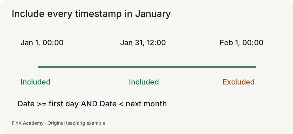
=SUMIFS(G5:G16,C5:C16,">="&J3,C5:C16,"<"&EDATE(J3,1))

The lower bound includes January 1. The exclusive upper bound excludes February 1 while including every timestamp on January 31. EOMONTH(J3,0) returns the month’s last calendar date; it is useful for labels, but a <= comparison to that midnight excludes later times on the final day.

State the fiscal convention

If a business starts its fiscal year in July and names the year by its ending year, July 2026 belongs to FY2027. With a date in C5, =YEAR(C5)+IF(MONTH(C5)>=7,1,0) produces that fiscal-year label. June 2026 belongs to FY2026. A different naming convention needs a different label, even though the underlying dates are unchanged.

Avoid using month names alone as keys across multiple years. January 2026 and January 2027 must not collapse into one month unless the task explicitly asks for a seasonal comparison.

Practice and check

Clean a product key containing ordinary spaces, parse 2026-02-28, and test the January filter with January 31 noon and February 1 midnight. Label June 30 and July 1, 2026 under the July-start convention.

Answers and reasoning

TRIM removes the ordinary surrounding spaces. The parsed date is February 28, 2026. January 31 noon is included and February 1 midnight is excluded. The fiscal labels are 2026 and 2027, respectively. Store the dates themselves alongside any fiscal labels so the classification remains traceable.

Transfer: import a file with a different date format. Document the new parsing rule and test an impossible date, a missing date and a year boundary before using its totals.

7. Build an expandable, readable report

Northstar adds a new sale beneath a fixed range. The total still looks reasonable because the new row is outside the formula. A reusable report needs an explicit way to include new data.

Outcome: use an Excel Table, understand structured references and recognize where dynamic arrays need a compatible application. Prerequisite: lessons 1–6. Environment: this is a native Excel lab; browser formula grading does not assess these interface actions.

Make the data rectangular

Use one row per transaction line, one header row, and one kind of value per column. Keep blank separator rows, merged cells, manually inserted subtotals and decorative headings outside the table. Save the original source before editing.

Select the sales range, choose Insert → Table, and confirm that it has headers. Name the table Sales. Give its columns meaningful names: Order, Date, Region, Product, Units, Price, Status and Revenue. A table is a structured data range; a PivotTable is a separate summarization tool.

In the Revenue column use =[@Units]*[@Price]. The @ indicates the current row. =SUM(Sales[Revenue]) sums the table’s Revenue column. The formula states its meaning without requiring the reader to remember a column letter.

Add a new sale at the bottom. Check that the table expands, the calculated-column formula reaches the new row and the total includes it. Do not assume that every imported paste or surrounding layout expands correctly. If a formula has been overridden in one row, inspect that exception before relying on the column.

Filters change visibility, not every calculation

Filter Region to North. An ordinary SUM over the table still includes filtered-out rows. For a visible-row total use =SUBTOTAL(109,Sales[Revenue]) in a location outside the data column. The 109 option sums visible cells while excluding filtered-out and manually hidden rows.

Keep both meanings clear: the complete eligible total and the currently visible filtered total answer different questions. A screenshot with a filter active can mislead a reader who assumes it shows the full business. Record the filter state in the handoff and clear it when appropriate.

Dynamic arrays are useful when supported

In a compatible modern Excel version, =SORT(UNIQUE(Sales[Region])) creates a list that expands from one formula cell. =FILTER(Sales,Sales[Region]="North","No matching rows") extracts North records. These are optional desktop extensions; check your installed Excel version before choosing them for a shared workbook.

Place a spilling formula outside the Excel Table and leave its output area empty. A value blocking the spill area can produce #SPILL!. Edit the formula at its anchor rather than typing over an individual spill result. Dynamic output is not permission to delete duplicates blindly: UNIQUE removes repeated values from its output, not necessarily invalid transactions from the business source.

If these functions are unavailable, use the table’s filters and a carefully maintained summary list with SUMIFS. That is a supported alternate learning route, not evidence that a browser grader has tested a spill operation.

Make the output usable

Put a clear title, currency and reporting period above the summary. Use separate formats for counts, money and percentages. Show unresolved mappings beside the affected output. A report with a missing category should not look complete simply because the grand total reconciles.

Before exporting or printing, inspect the preview. Set an appropriate print area and repeat table headers on long pages. Fit to one page wide if readable; do not force hundreds of rows onto one page tall. Confirm that negative amounts, long labels and the period are visible. A CSV stores flat data, not the workbook’s formulas, multiple sheets, formatting or charts; use XLSX when those need to survive.

Practice and check

Create three clean rows: North sells 10 units at $30, South sells 8 at $45, and North sells 15 at $30. Convert the range to Sales, add Revenue, and append a North sale of three units at $20. Filter to North. Compare SUM and SUBTOTAL, then remove the filter and save the XLSX.

Expected behavior

The added line contributes $60. The table and formula column should expand. SUM includes every table row; SUBTOTAL changes with visible rows. A spilled region list, when available, updates if the new sale introduces a region. The exported workbook should retain formulas after reopening.

Transfer: add another transaction after reopening the file. Check expansion again and explain which parts of the report update automatically and which require refresh or manual range maintenance.

8. Sort, pivot and chart in native Excel

A report can calculate the right total and still show the wrong relationships if one column was sorted independently. Keep each transaction’s fields together as you explore it.

Outcome: produce a checked monthly sales report using native Excel sorting, filtering, a PivotTable and a chart. Prerequisite: lessons 1–7. This is a self-reviewed desktop lab. A FinX numerical exercise pass does not establish that these features were created or reviewed.

Download the sales practice workbook and complete the cleanup rules in lesson 9 before building the PivotTable. Work on a copy. The workbook includes the raw source and a workspace; it does not pre-complete the pivot for you.

Preserve the row relationship

In the cleaned table, select a cell and sort by Date ascending, then Order ascending. Use the table’s sort or select the full data range. Do not sort the Date column alone. Check one named order before and after: S006 should still have 20 units, a $30 price and a February 5 date.

Filter to February and inspect the records, including the return. A negative return belongs in net sales under this case’s policy. Removing it because it makes a chart less attractive changes the business definition.

Build the pivot from eligible records

After removing the one confirmed duplicate and excluding the canceled order, create an Excel Table from the eligible records and name it EligibleSales. Add Revenue as Units × Price and Month as the first day of the transaction month. Insert a PivotTable from that table.

1. Put Month in Rows.
2. Put Region in Columns.
3. Put Revenue in Values and confirm the aggregation is Sum.
4. Format the values as USD and the month labels as month plus year.

If Excel offers Count of Revenue, inspect whether the field contains text or mixed types. Changing Count to Sum without fixing the source can leave missing numeric values unnoticed. Reconcile the pivot’s grand total to the independently checked eligible source total.

Month, 2026	North USD	South USD	Total USD
January	660	360	1,020
February	30	800	830
March	450	100	550
Total	1,140	1,260	2,400

North February includes a $120 shipment and a -$90 return. March includes $100 for unmapped product X because the supplied units and transaction price are valid. The category report must expose that exception, as lesson 9 explains.

Chart the comparison the reader needs

Create a clustered column chart for the three monthly total sales figures. Title it Northstar net sales, January–March 2026 (USD). Use a zero baseline for these positive column lengths, chronological months and readable labels. Exclude the grand-total row from the plotted months. Do not mix unit counts and dollars on one unlabeled axis.

The chart should make January’s 1,020, February’s 830 and March’s 550 easy to compare. It does not prove a trend will continue or explain causation. The source contains only a small fictional teaching sample.

Refresh is a separate behavior

Change S006 from 20 to 22 units in your working source. Its revenue should rise by $60. Refresh the PivotTable. February should become 890, South 1,320, and the grand total 2,460. Check the chart as well. Then restore 20 units and refresh again. A pivot showing the old total can be stale even while the underlying worksheet formulas have updated.

Save evidence of your work

Save an XLSX containing the formula-driven clean table, pivot and chart. Reopen it, inspect the formulas and refresh. Use print preview to check labels and legibility. Record your Excel version, whether dynamic arrays were available, the changed-input results, and any manual steps needed to include new rows.

Self-review checklist: the whole record survived sorting; the duplicate and cancellation policies are documented; the return remains negative; pivot values use Sum; the total reconciles to 2,400; the chart uses the three months; the changed-input test passes; the restored file returns to 2,400. A tutor can review this evidence separately. No independent review or credential is implied by ticking your own checklist.

9. Case: turn an unfamiliar sales file into a checked report

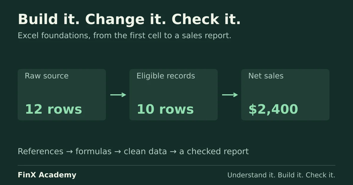
You receive twelve rows from Northstar’s sales export. The manager asks for net sales by month and region, plus a product-category breakdown. There is a repeated order, a cancellation, a return, a text quantity, a padded product key and an unmapped product. Your job is to preserve the source, apply documented rules and make the unresolved exception visible.

Outcome: combine cleanup, formulas, conditional summaries and lookup diagnosis in one traceable report. Prerequisite: lessons 1–7; complete lesson 8’s pivot and chart after preparing this case’s source. This is an open learning case with solutions, not an unseen certification assessment. Attempt it before expanding the solution.

Source pack and policy

Use the practice workbook, raw CSV and product mapping. Each row is an order line. Dates are valid ISO calendar dates in 2026. Quantities are units; prices are USD per unit and revenue is USD. Prices are transaction prices, not values to replace from the product map.

Rule	Treatment
Duplicate S006	Two identical exported rows represent one order line. Retain the first and record the removed copy.
S004 cancellation	Exclude it from recognized net sales. Keep it in the audit trail.
S007 return	Include its negative units and negative revenue in February.
Product A	Remove ordinary surrounding spaces in a derived column.
Quantity text 12	Convert to numeric under the supplied integer-unit convention.
Product X	No category mapping exists. Include its known transaction revenue and show Unmapped in the category report.
S011 zero units	Valid record. Keep it; zero activity is not missing data.

Order ID is unique in this case after removing the confirmed duplicate. In another business, one order could contain many line items, so removing repeated order IDs would destroy legitimate sales. Do not generalize this policy without establishing the source grain.

Your task

Keep the Raw sales sheet unchanged. In Working sales, link the source fields, create cleaned product, numeric units, a real date, eligibility and revenue columns. Keep a disposition note for the duplicate and canceled rows. Build a monthly-by-region summary using SUMIFS with date boundaries, or create a first-of-month key and aggregate on that key.

Check product-map uniqueness before retrieving categories. Missing category information does not make the known sale price zero. Show mapped revenue and unmapped revenue separately so the breakdown adds back to the same total. Write two sentences explaining what can be concluded and what still needs a source correction.

Reconcile the report in three ways: monthly totals to the eligible transaction total; regional totals to the same total; category totals including Unmapped to the same total. Add a duplicate and exception count. A reconciliation using the same mistakenly duplicated source on both sides is insufficient, so also inspect the named duplicate’s disposition.

Progressive hints

Hint 1: sort or filter a working copy by Order to inspect S006. Do not overwrite the raw export. Mark the duplicate before calculating a report.

Hint 2: establish numeric units and valid dates before aggregating. Separate the eligibility rule from the price × units calculation. Preserve the return’s sign.

Hint 3: use an inclusive first-of-month and exclusive next-month boundary. For categories, count each key’s matches in the master, then retrieve only an unambiguous mapping. Use an explicit Unmapped bucket for X under this case’s policy.

Solution and independent reconciliation

There are 12 raw rows, 11 unique order lines after removing one duplicate copy, and 10 included lines after excluding S004. Included net units are 83. A zero-unit included line still counts as one included record.

Month	North USD	South USD	Net sales USD
January	660	360	1,020
February	30	800	830
March	450	100	550
Total	1,140	1,260	2,400

An independent transaction sum is 300 + 360 + 360 + 120 + 600 − 90 + 200 + 450 + 100 + 0 = 2,400. The canceled $225 and duplicate $600 are excluded. Summing all raw transaction amounts would produce 3,225, which is 825 too high.

Product A contributes 1,710, B 270, C 320, and X 100. The mapping puts A and B in Drinkware and C in Accessories. Thus Drinkware is 1,980, Accessories 320, and Unmapped 100. Known-category revenue is 2,300; it must not be presented as the full 2,400.

One suitable handoff is: “Net sales for January–March are $2,400 after removing the confirmed duplicate and canceled line, including a $90 return. Product X accounts for $100 of that total and still needs a category mapping; the category report shows it separately as Unmapped.”

Prove that the model responds

Change only S006’s working quantity from 20 to 22. February and South should increase by $60; total sales should become 2,460. Restore it. Then temporarily remove C’s category mapping: total revenue must remain 2,400, while Unmapped revenue increases from 100 to 420. Restore the mapping and refresh any pivot.

These tests address different risks. The first catches hardcoded outputs. The second catches a lookup fallback that quietly drops revenue. Also inspect the first and last transaction formulas, not just one middle row.

Transfer and review

For a later retry, ask a tutor to provide a different source with a genuine multi-line order and a price-effective-date mapping. That changes the relationship, not just the numbers. This public case cannot supply evidence of unseen performance.

Review numerical accuracy, source traceability, behavior after edits, and the clarity of the exception explanation separately. Desktop features and written judgment require self-review or a named reviewer. Continue with accounting and source-data reconciliation once you can explain why each included row belongs in the report.

Primary documentation and further practice

Microsoft documentation checked 7–8 October 2026. Function behavior and feature availability should be checked in the learner’s installed application. The course examples, datasets, diagrams and explanations are original FinX teaching material.

• Formula references: how references connect cells and change when copied.
• XLOOKUP: exact matching, first-match behavior, missing matches and availability limitations for Excel 2016/2019.
• Conditional sums: SUMIFS criteria and argument order.
• Diagnosing #N/A: missing keys and type mismatches.
• Sorting a range or table: sorting and recognizing text dates.
• TRIM: ordinary spaces and the character-160 limitation.
• Dynamic arrays and spilling: spill areas, blocked outputs and placement outside Tables.
• PivotTable sources and refresh: rectangular source data, source Tables and refresh behavior.

The downloadable workbook is an editable learning scaffold. The solutions are deliberately public. Neither completing the written case nor passing a numerical drill establishes independent mastery of native Excel tables, pivots, charts or written judgment.