Revenue forecasting: build a price-and-volume driver model

A revenue forecast built by typing “8%” next to last year’s number predicts a total. A driver-based forecast — volume × price, month by month — predicts the shape as well, and every input can be owned, dated and challenged. This page builds one for twelve months of 2027 for the same regional industrial-maintenance business the comps article and the precedent-deals article value: a separately supplied 2026 full-year revenue assumption of 315.0 and the comps example’s LTM EBITDA of 45.0. Those periods differ; do not divide them into a reported margin. All operating drivers below are new fictional assumptions, not figures derived in the valuation articles. Amounts are in millions of one currency. Revenue only: costs, EBITDA and the statements below revenue are out of scope here, beyond saying where this schedule plugs in.

Start from the answer a growth rate hides

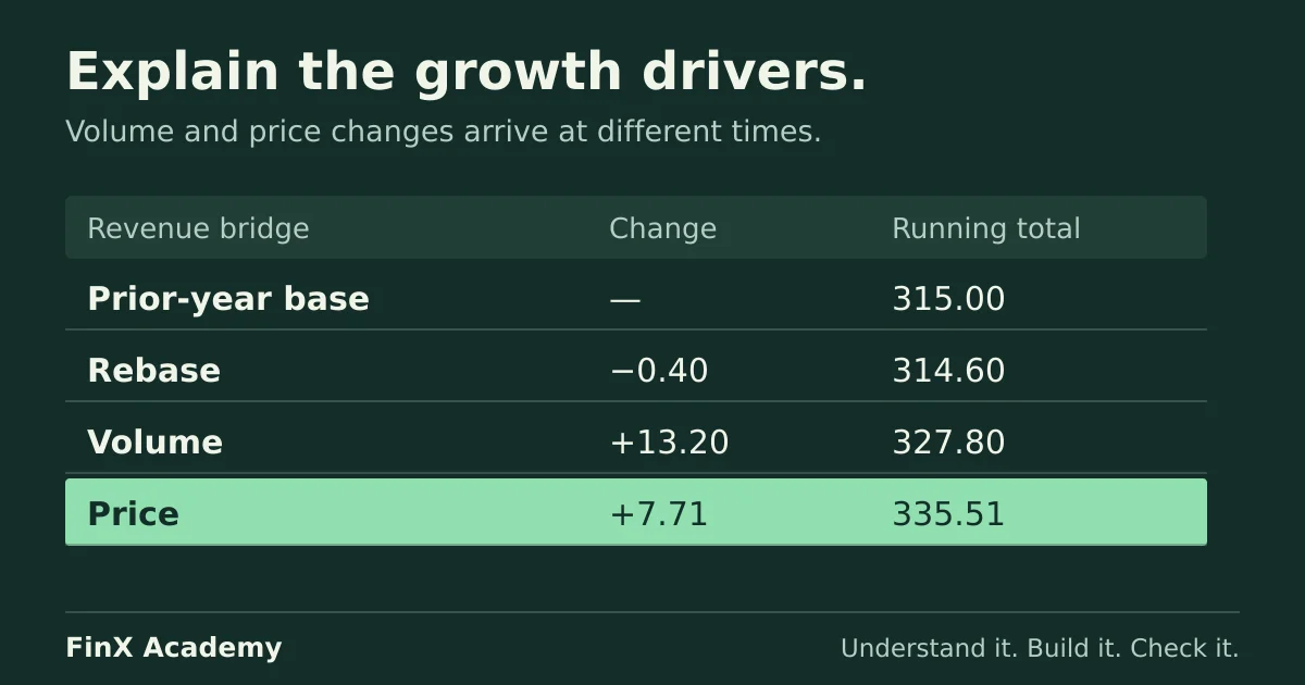
The finished model grows 2026 revenue of 315.0 to 335.5, which is +6.5%. The point is not the 6.5 — it is what the number decomposes into:

Bridge step	Amount	Running total
2026 full-year revenue assumption		315.0
Rebase to 240 contracts all year plus the stated job plan	−0.40	314.60
Volume: 2 net new contracts per month at the old fee	+13.20	327.80
Price: 5% uplift billed from July	+7.71	335.51

The first adjustment is an explicitly unresolved difference from the prior-year assumption, not a fabricated volume effect. A real budget needs the 2026 contract and job history to explain it. The forecast decisions are: contracts won per month, and a repricing date. A single “8%” says neither — and it is not even the same question: the growth rate of the year hides that December total (29.1) is higher than January’s (25.8) while December’s non-recurring job revenue (1.6) is the lowest of the year. The smooth-looking total conceals a soft, seasonal line most months the total never shows.

Enter the drivers, one convention at a time

Months across the top (B3:M3, Jan–Dec 2027), labels in column A, annual in N:

Row	Label	Jan	Feb	Mar	Apr	May	Jun	Jul	Aug	Sep	Oct	Nov	Dec
4	Opening contracts	240	242	244	246	248	250	252	254	256	258	260	262
5	Net additions	2	2	2	2	2	2	2	2	2	2	2	2
6	Closing contracts	242	244	246	248	250	252	254	256	258	260	262	264
7	Fee per contract (millions)	0.100	0.100	0.100	0.100	0.100	0.100	0.105	0.105	0.105	0.105	0.105	0.105
8	Recurring revenue	24.00	24.20	24.40	24.60	24.80	25.00	26.46	26.67	26.88	27.09	27.30	27.51
9	Jobs planned	45	45	50	55	60	65	70	70	65	55	45	40
10	Avg invoice (millions)	0.040	0.040	0.040	0.040	0.040	0.040	0.040	0.040	0.040	0.040	0.040	0.040
11	Job revenue	1.80	1.80	2.00	2.20	2.40	2.60	2.80	2.80	2.60	2.20	1.80	1.60
12	Total revenue	25.80	26.00	26.40	26.80	27.20	27.60	29.26	29.47	29.48	29.29	29.10	29.11

The formulas, entered once and copied across:

Cell	Formula	Convention it encodes
C4	=B6	The roll-forward: this month opens where last month closed. Only B4 is typed.
B6	=B4+B5	Closing = opening plus net adds, nothing else — cancels belong in B5
B8	=B4*B7	Opening contracts × monthly fee: net additions start service and billing next month
B11	=B9*B10	Non-recurring line: planned jobs × average invoice, its own drivers
B12	=B8+B11	Two engines, one total — never a third “adjustments” row inside it

B4 is 240 and B5 is 2. Opening contracts, net additions, service-start timing, price uplift, effective date, job counts and average job value are all assumptions requiring support. A real build sources them the way every other line on this site sources its inputs — booked-contract report for the additions, signed price list for the uplift, both dated. Three points of discipline to state before anyone asks:

• Unit labels live in the row label. Rows 7 and 10 are millions per contract per month and per completed job; rows 8 and 11 are millions in the month. A model whose 0.100 might be a fee or a fee-times-twelve is one careless copy away from a unit-scale error.
• One revenue definition. We assume service starts next month, is delivered evenly during each active month, and is billed in that same month; each planned job is completed and recognised in its listed month. Invoicing alone does not establish revenue recognition. IFRS 15 ties recognition to satisfying performance obligations. If starts and cancellations have different timing, model them separately instead of using a single net-additions row.
• The uplift is dated, not annualised. Row 7 changes the fee cell from its effective month. Spreading the 5% across all twelve months instead overstates the year by the first-half contract-months that weren’t charged: 1,470 × 0.005 = 7.35 — and the bounds test below is calibrated to catch exactly that.

Reconcile before you trust it

For annual flow totals use =SUM(B8:M8) in N8 and =SUM(B11:M11) in N11; N12 is =SUM(B12:M12). Do not sum contract balances into an annual closing balance: that is M6.

One route: the twelve months sum to the year. A second, independent route: the lines do.

1. =SUM(B12:M12) → 335.51, and =N8+N11 → 308.91 + 26.60 = 335.51 ✓. Same total from months or from product lines; a mismatch means a row is missing or double-counted.
2. Roll-forward check: =M6 (Dec closing, 264) must equal =B4+12*B5 (240 + 24 = 264) ✓. The cumulative view recomputes the chain from its two drivers instead of trusting twelve chained copies.
3. Bounds: with nothing growing and no uplift the model still earns 240 × 12 × 0.1 + 26.6 = 314.6 — 0.40 below the prior-year assumption. Closeness is a reason to investigate, not a completed back-test; the actual prior-year contract and job data have not been supplied. With the uplift effective all twelve months it could not exceed 3,012 × 0.105 + 26.6 = 342.9. The answer 335.51 sits inside the band ✓; 342.9 would mean billing a price rise for months it wasn’t charged.
4. Bridge: 315.00 − 0.40 + 13.20 + 7.71 = 335.51. Volume is (3,012 − 2,880) × 0.100 = 13.20; price is 1,542 × 0.005 = 7.71. This sequential bridge assigns the volume/price interaction to price. The −0.40 baseline difference remains visible until historical drivers explain it.

A driver change is computable; a hardcode is only re-guessable

Commercial asks for net adds of 3 per month instead of 2, for twelve extra contracts across 2027. The model’s answer: +6.855 (total 342.365). The intuition that reaches for 12 × 0.1 × 12 = 14.4 has already doubled the truth, because it bills every arrival for a full year. An addition bills only from the month after it joins: the January cohort bills eleven months (1.13), one arriving in February bills ten (1.03), the November cohort bills a single month (0.105) and the December cohort bills nothing in 2027. Summing the twelve cohorts — 1.13, 1.03, 0.93, …, 0.105, 0 — gives 6.855, and the pattern is the lesson: an addition is worth a year of fee at the start of the horizon and nothing at the end.

The same discipline prices a second hypothetical decision: cut the uplift from 5% to 3% and the effect is 1,542 opening-contract-months × 0.002 = −3.084. Against a top-down =315*1.08 hardcode — 340.2, already +4.69 above the bottom-up answer — there is no July cell to renegotiate; you re-guess a percentage and learn nothing about why the guess moved. (If leadership insists on their number, don’t overwrite the drivers — record 340.2 beside 335.51 and make the 4.69 defend its contract wins.)

Break it and trace the effect

1. A broken roll-forward. Type 240 into C4 instead of =B6, copy across, and contracts never grow: recurring revenue flattens, the year lands on 321.8, understated by 13.71 (−4.1%) — and every monthly number looks perfectly smooth, which is why nobody spots it by eye. The roll-forward check catches it in one glance: M6 says 242, B4+12*B5 says 264. Chained references need a cumulative witness for exactly this reason — the absolute-reference guide is the same story on a smaller sheet.

2. Multiplying the wrong contract row. Replace =B4*B7 with =B6*B7 and every month bills the contracts that join during it as if they had arrived on the first. The year rises only +2.46 — small enough to ship — but the convention has silently become “arrivals bill immediately”, the answer nobody sourced. Anchor on the first month: January recurring must be 240 × 0.100 = 24.00; if it reads 24.20, row 8 references the wrong row.

3. The uplift leaks into the jobs line. Apply the July 5% uplift to both recurring revenue and jobs, when only the contract fee changes, and H2 job revenue is overstated by 13.80 × 5% = 0.69. The total becomes 336.20. Applying it to jobs for all twelve months would instead add 1.33; those are different errors. Compounding discipline is the CAGR guide’s subject; the lesson here is narrower — a price decision lives in the price row, on its effective date, nowhere else.

Check your answers

• Monthly totals Jan–Jun 25.80, 26.00, 26.40, 26.80, 27.20, 27.60; Jul–Dec 29.26, 29.47, 29.48, 29.29, 29.10, 29.11. Annual: recurring 308.91, jobs 26.60, total 335.51.
• Bridge: 315.00 − 0.40 baseline difference + 13.20 volume + 7.71 price = 335.51; bounds 314.6 ≤ 335.51 ≤ 342.9; roll-forward 264 = 240 + 12 × 2.
• Growth +6.5%; adds-only case 327.8 (+4.1%); uplift contributes a further +2.3%.
• Driver changes: adds 3/month → 342.365 (+6.855), not the naive 14.4; uplift at 3% → −3.084.
• Breaks: flat chain → 321.8 (−13.71); closing-row multiply → +2.46; hardcode → 340.2 (+4.69).

Take the next step

Revenue is the top row of the three-statement model: the income statement inherits it and everything else cascades down. The working-capital schedule turns forecast credit sales into receivables; both price and volume changes affect the amount to collect, and the scenario-analysis guide is the machinery for running the adds-and-pricing cases as base, upside and downside instead of one hero number. FinX’s Three-Statement Build course provides structured spreadsheet practice; browse the catalogue for the current syllabus. The free ten-minute diagnostic asks five numeric modelling questions; it does not grade a driver build. The full Three-Statement Build course requires paid access.

Keep the approved plan alongside each dated expectation using the budget vs forecast worked example.